Plot

Module 7.2: Measurement Error
All materials can be found at alexcardazzi.github.io.
In each of the models we’ve estimated thus far, we’ve included an error term. Error terms are, effectively, all the other things we cannot observe or account for that still affect the outcome, as well as sheer randomness.
Sometimes in social science, business, etc., we are unable to perfectly measure our variables, which we call measurement error. Measurement error can arise for many different reasons such as sampling error, numbers being rounded or truncated, misreporting, etc.
What are the effects of measurement error?
Measurement error in explanatory variables biases coefficients towards zero. Note the difference between this and omitted variable bias. Omitted variable bias pushes coefficients in a specific direction (positive or negative). If the omitted variable bias is negative, true negative coefficients become more negative and true positive coefficients become less positive.
True positive coefficients can even become negative altogether. See the bedrooms and square footage example from Module 5.
However, with measurement error in explanatory variables, coefficients get squished down towards zero rather than pushed up or down.
Random measurement error in \(Y\) gets absorbed into the error term. In reality, this just makes inference more difficult (by increasing the standard errors of the coefficient estimates).
As a broad, descriptive summary, measurement error in \(X\) variables will bias coefficients towards zero. Measurement error in \(Y\) does not bias your coefficients, but does inflate their standard errors. In the following, I will demonstrate some of the effects of measurement error using some simulated data.
In this section of notes, I have simulated two datasets of 50 observations each. Both datasets are simulated exactly the same way, except at different times so the random numbers will be different. The data is generated by:
\[Y_i = X_i + e_i\]
To generate measurement error in \(X\), I create a new variable called \(\widetilde{X}\), which is simply \(X\) plus some random noise that progressively gets larger. To generate measurement error in \(Y\), I slowly increase the magnitude of the error term \(e\) in the equation above. The figures below are gifs that demonstrate what happens as measurement error in either \(X\) or \(Y\) increase.


In the panel on the left, you’ll see that the points spread out horizontally but do not change their vertical positions. Notice how the regression line, depicted in solid black, seems to quickly flatten out as the measurement error increases. This is what I mean by saying measurement error in \(X\) pushes the slope coefficient towards zero.
In the panel on the right, the opposite movement is occurring for the points. Here, they are spreading out vertically, but not changing their position horizontally. In this example, the regression line becomes more vertical over time (i.e., the slope coefficient is pushed away from zero), but this is due to the particularities of this specific simulation. With measurement error in \(Y\), the slope coefficient is as likely to increase as it is to decrease.
See below for the second set of simulations with similar results.


The following figure tracks both the coefficient estimates and standard errors for a similar simulation as measurement error increases. Again, the slope coefficient plummets towards zero as measurement error in \(X\) increases, whereas the effect of measurement error in \(Y\) is much less stark. However, the opposite is true for the standard error estimates. While the coefficient heads towards zero while measurement error in \(X\) increases, the standard error also decreases. At first glance, this might look like precision is improving, but it is not good news: the coefficient is shrinking much faster than its standard error. What matters for inference is the size of the coefficient relative to its standard error, and that ratio is getting worse. This ratio is exactly how we calculate a t-statistic (see Module 4.4): \(t = \widehat{\beta} / se_{\widehat{\beta}}\). On the other hand, while the coefficient estimate is less affected by measurement error in \(Y\), the standard error steadily climbs.
To put numbers on this: with no measurement error in \(X\), the t-statistic is 6.0. With the most measurement error, the standard error is smaller than it started (0.04 compared to 0.16), but the t-statistic has collapsed to 0.7.
Generally speaking, you will be unable to determine exactly how much measurement error you are dealing with and whether it is in \(X\), \(Y\), or both. Typically, people will mostly write things like, “this estimate is a lower bound, since measurement error is pushing the coefficient towards zero.” Or, “the estimate is insignificant, but this may be due to measurement error in the outcome variable.” Do these arguments work? Sometimes. Like most things, it really just depends.
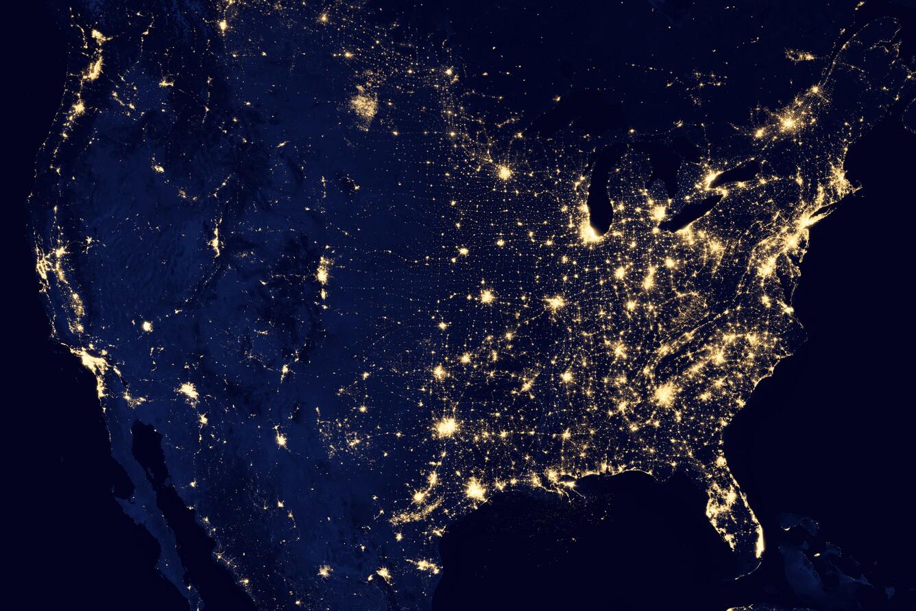
Another point worth making is that these simulations only consider random measurement error rather than non-random error. Random error is when measurements are equally likely to be high relative to low. However, measurement error is considered non-random when the measurements are consistently, or more likely to be, inflated or deflated. Take this article from The Economist as an example. Some clever economists got their hands on satellite data that measured how bright a given country or city was at night. Their hypothesis was that areas with more economic activity should have more ambient light at night compared to less developed areas. As a simple example, see this image of the United States at night. Anyway, these economists used luminosity to predict GDP, and found that autocratic countries consistently reported higher levels of GDP than what their luminosities would suggest. This was not the case for democratic countries. The point here is that this represents non-random measurement error in reported GDP.
Non-random measurement error can be thought of as a form of omitted variable bias. In this example about GDP and luminosity, we can also observe levels of freedom within a country, which can therefore be used as a control. However, if low GDP countries inflated their reported GDPs but high GDP countries did not, then using this variable in a model would not be particularly helpful.