In the last lecture, we used the CLT to build a confidence interval around a sample mean. Here, we use the same machinery to test a hypothesis.
Heart Medication
Suppose we are working for a large pharma company. This company has recently released a new drug that they think will increase heart rates. This is our hypothesis. To test this, we are going to do the following:
To start, we will measure the heart rates (\(\text{HR}\)) of 100 individuals as a baseline.
We’ll then give these 100 individuals the heart medicine, and re-measure their heart rate.
For each person, we will calculate the change in their heart rate.
From now on, the data I will use is \(\text{HR}_{\text{drug}} - \text{HR}_{\text{baseline}}\), the mean of which is \(\hat{y}\)
Now, if we assume that our drug does not work, we would expect \(\mu = 0\) and \(\hat{y} \approx 0\). In English, heart rates should not increase if the drug is ineffective. Essentially, we are going to make a confidence interval around 0. Then, if we find \(\hat{y}\) is outside of that confidence interval, we can reject the idea/assumption/hypothesis that the drug is ineffective.1
If \(\hat{y}\) is outside the null hypothesis’s confidence interval, we say we reject the null. In other words, we have found evidence to rule out the null hypothesis. Be careful: evidence \(\neq\) proof.
If \(\hat{y}\) is inside the null hypothesis’s confidence interval, we say we fail to reject the null. In other words, we have not found strong enough evidence to rule out the null. We never say that we accept the null hypothesis. Why the double negative? In statistics, the absence of evidence is not evidence of absence.
The next step would be to construct this confidence interval around zero. We need three things:
A center for the interval. This one is easy: it’s zero
A confidence level. This one is arbitrary: let’s use 95%, or \(z = 1.96\)
A standard error. This one is calculable: \(\frac{s}{\sqrt{n}}\)
Once we construct our interval, we must come up with critical values. This is just a fancy term for the edges of our confidence interval. Here, the critical values are:
Finally, if \(|\hat{y}| > 1.96 \times \frac{s}{\sqrt{n}}\), or in words, the magnitude of the sample mean is greater than the critical value, we can reject the null. Otherwise, we fail to reject the null. Dividing both sides by the standard error, this is the same as checking whether \(|\sqrt{n} \times \frac{\hat{y}}{s}| > 1.96\), or in words, whether the magnitude of the test statistic is greater than 1.96. The test statistic is measured in standard errors, which is why it is compared to \(z = 1.96\) rather than to a critical value in heart rate units.
Let’s simulate some data and see what happens. Assume the baseline heart rate average is 80 beats per minute and the “drugged” heart rate is 82 beats per minute. Can we say that the drug worked? Numerically, heart rates seem to have increased! However, this could just be due to random chance. We need to figure out how likely this number would be assuming the medication does not work.
Code
hr_before <-rnorm(n =100, mean =80, sd =5)hr_after <-rnorm(n =100, mean =82, sd =5)hr_diff <- hr_after - hr_beforehr_diff_mean <-mean(hr_diff)hr_diff_sd <-sd(hr_diff)hr_diff_n <-length(hr_diff)cat("Mean of Difference in Heart Rate:", hr_diff_mean, "\n")cat("St. Dev. of Difference in Heart Rate:", hr_diff_sd, "\n")cat("Sample Size of Difference in Heart Rate:", hr_diff_n)
Output
Mean of Difference in Heart Rate: 1.946905
St. Dev. of Difference in Heart Rate: 6.299079
Sample Size of Difference in Heart Rate: 100
Our critical value is: \(1.96 \times \frac{s}{\sqrt{n}}\)
Our test statistic is: \(\sqrt{n} \times \frac{\hat{y}}{s}\)
Code
critical_value <-1.96* (hr_diff_sd /sqrt(hr_diff_n))test_statistic <-sqrt(hr_diff_n) * (hr_diff_mean / hr_diff_sd)cat("Sample Mean:", hr_diff_mean, "\n")cat("Critical Value:", critical_value, "\n")cat("Test Statistic:", test_statistic, "\n")# These two rules are equivalent:# (1) the sample mean vs. the critical value (both in heart rate units)# (2) the test statistic vs. 1.96 (both in standard errors)# abs() is used because a sample mean far below zero is just as extreme.if(abs(hr_diff_mean) > critical_value){cat("Reject the Null")} else {cat("Fail to Reject the Null")}
Output
Sample Mean: 1.946905
Critical Value: 1.234619
Test Statistic: 3.090778
Reject the Null
Our hypothesis test suggests that we should reject the null hypothesis, or in other words, it is unlikely that the null hypothesis is true. However, comparing two numbers might not be particularly intuitive.
Below is a visualization of the entire distribution of the sample means we would expect IF the null was true. The shaded region represents where we would expect 95% of those sample means to fall. The red vertical line represents what we observed in the data.
Plot
But, isn’t this entirely arbitrary? Consider the plot below. Given our previous steps, we would treat each one of these red lines the same as one another even though they’re all different distances from the critical value.
Plot
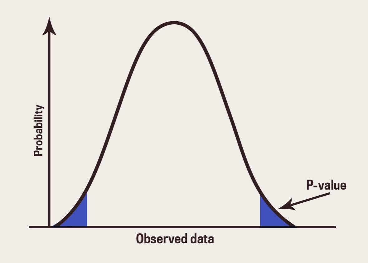
This is why statisticians came up with the idea of something called p-values.
Tip\(p\)-value
A \(p\)-value represents the probability of observing a sample value as extreme as, or more extreme than, the value observed, given the null hypothesis is true.
\(p\)-values are misinterpreted by even the most experienced researchers, and they take a lot of time to grasp. It’s a crucial concept, though, so make sure to take the time to think about this. We will be dealing with p-values (and test statistics) through out the rest of this course.
To calculate a p-value, we need to figure out the probability mass to the right of the positive test statistic plus the probability mass to the left of the negative test statistic. See here for an example. Calculating one of the two ranges in R is easy. To calculate the area of both, we can just multiply by 2.
Code
2*pnorm(abs(test_statistic), lower.tail =FALSE)
Output
[1] 0.00199633
This section of the module contained a lot of statistical theory and coding. However, the point was to have you go through this so you understand deeply the concept of hypothesis testing before you were exposed to some of the shortcut functions.
Of course, R contains some handy functions for hypothesis testing. See below for some of these.
Code
# Note the output of this function.# There is a "mean", "t", and "p-value"# The "mean" and "t" are exactly equal to# what we calculated before.# The "p-value" is slightly different# but the reason is unimportant for now.# R also generates a 95% conf. interval for you.# Note, though, that this is different from what had.# Again, this is unimportant for the moment.t.test(hr_diff)cat("\n\n")# You can use the following code for the same output.# paired = TRUE effectively differences the data for you.# Note, I am changing the confidence level to 99%t.test(hr_after, hr_before, paired =TRUE, conf.level =0.99)cat("\n\n")# You can also compare two independent samples# These can even have different sample sizes.# For example, a prof might want to know if# two classes scored statistically differently on# on an exam. This would be how to do that.# Everything would be interpreted in the same way.# You might notice that some of the output is different# when doing the analysis this way.t.test(hr_after, hr_before, paired =FALSE)
Output
    One Sample t-test

data:  hr_diff
t = 3.0908, df = 99, p-value = 0.002593
alternative hypothesis: true mean is not equal to 0
95 percent confidence interval:
 0.6970314 3.1967790
sample estimates:
mean of x
 1.946905


    Paired t-test

data:  hr_after and hr_before
t = 3.0908, df = 99, p-value = 0.002593
alternative hypothesis: true mean difference is not equal to 0
99 percent confidence interval:
 0.2925118 3.6012986
sample estimates:
mean difference
       1.946905


    Welch Two Sample t-test

data:  hr_after and hr_before
t = 2.9426, df = 197.63, p-value = 0.003644
alternative hypothesis: true difference in means is not equal to 0
95 percent confidence interval:
 0.6421451 3.2516653
sample estimates:
mean of x mean of y
 81.99224  80.04534
Footnotes
It is equivalent to think about this process as building a confidence interval around \(\hat{y}\) instead, and then checking if 0 is or is not inside that interval. In fact, the width of these intervals will be the same, the only thing that changes is the center. Due to this, the conclusions you draw will be identical.↩︎