Plot

Module 3.1: Probability and the Normal Distribution
All materials can be found at alexcardazzi.github.io.
So far, we have summarized data with its mean, variance, and overall distribution. To use these ideas to say something about a whole population from a sample, we first need some probability.
A value between 0 and 1 inclusive that represents the likelihood a particular event happens.
The probability that a coin is flipped and it lands on tails is \(\frac{1}{2}\) or \(0.5\) or \(50\%\). What about the probabilities and outcomes of flipping two coins and counting the number of tails? Well, since flipping this coin is a random variable, it has a distribution. That distribution is defined by all possible outcomes and the associated probabilities:
Percentages are not really probabilities, but they are often associated with them.
| Number of Tails, \(y\) | Probability, \(P(y)\) |
|---|---|
| 0 | 0.25 |
| 1 | 0.50 |
| 2 | 0.25 |
All distributions have a mean and a variance. So, how do we find the mean and variance of a probability distribution?
In fact, not all distributions have defined means and/or variances, but these types of distributions are outside the scope of this course.
\[ \mu = \sum_{i = 1}^g P(y_i) \times y_i \]
\[ \sigma^2 = \sum_{i = 1}^g P(y_i) \times (y_i - \mu)^2 \]
These formulas should look a lot like formulas for weighted averages!
To practice, let’s use the previous distribution of the number of heads from flipping two coins.
\[ \mu = \sum_{i = 1}^g P(y_i) \times y_i = (0.25\times0) + (0.5\times1) + (0.25\times2) = 1 \]
\[ \begin{aligned}\sigma^2 &= \sum_{i = 1}^g P(y_i) \times (y_i - \mu)^2 \\ &= (0.25\times(0-1)^2) + (0.5\times(1-1)^2) + (0.25\times(2-1)^2) \\ &= (0.25\times(-1)^2) + (0.5\times(0)^2) + (0.25\times(1)^2) \\ &= 0.25 + 0 + 0.25 = 0.5\end{aligned} \]
Flipping coins is an example of a discrete distribution. In other words, individual events have non-zero probabilities of occurring. However, when distributions are continuous, the probability of any individual event occurring is precisely zero. What? How can that be true?
Consider the lifespan of a tire on a car. Suppose the average tire lasts about 54,000 miles. However, what is the probability that your tire lasts exactly 54,000 miles? Essentially 0%.
This is because your tire could last 54,000.1 miles, 54,000.01 miles, and so on. There are an infinite number of miles that your tire could last, so the probability of any specific mile being the one where your tire goes flat is zero.
When dealing with continuous probabilities, instead of asking for the \(P(y) = M\) (e.g., the probability that your tire lasts exactly \(M\) miles), people ask for the \(P(y) < M\), \(P(y) > m\), or \(m < P(y) < M\) (e.g., the probability that your tire lasts more or less than some number of miles, or the probability that your tire lasts between two numbers of miles.)
In the interest of being concrete, suppose tires last anywhere between 40,000 and 68,000 miles. Suppose further that the distribution is uniform, meaning that the probability of your tire going flat is the same from 40,000 to 68,000 miles. A question from a statistics class might be: “what is the probability that your tire lasts more than 60,000 miles?”
To answer this, you need to know what fraction of tires last above 60,000. Well, since all tires go flat between 40 and 68, we can say the baseline is 68-40 = 28. Then, 68-60 is the range we’re interested in. So, the probability would be \(\frac{68-60}{68-40} = 0.286\).
The above math highlights how you would deal with probabilities and continuous distributions. However, not all continuous distributions are “uniform” like we assumed above. Perhaps the most famous and widely studied distribution is the normal distribution.
The normal distribution:
Below is an example of what a normal distribution looks like:
Normal distributions take on different shapes depending on their means and standard deviations.
Below are some examples of what these changes would do to a standard normal distribution:

To learn the most incredible feature of the normal distribution, you’ll have to wait for later in the module. However, while we wait, let’s discuss how to compare two different normal distributions.
Two particularly famous distributions that are normally distributed are scores on the SAT and ACT. The maximum score for each is 1600 and 36, respectively. The SAT has an average score of 1050 with a standard deviation of 200. The ACT has an average score of 19 with a standard deviation of 6.
So, let’s say someone scores a 1,300 on the SAT and a 29 on the ACT. Which test did they do better on?
Well, let’s first visualize the two distributions and the two scores.

Unfortunately, this visualization is not so helpful. Since the two distributions have different means and standard deviations, we cannot really compare them. A first step to getting a better comparison would be to subtract off the mean from both distributions. Then, both distributions will have a mean of zero.

Still, this is not helpful. Now, the variances are distorting the comparison. To fix this, we can divide each by their respective standard deviations. This way, both distributions have a mean of zero and a variance of 1.

Now, it should be quite obvious which score was “better”. The SAT score currently has a value of 1.25 while the ACT score has a value of 1.6666667.
What do these numbers mean, though? In words, this is the number of standard deviations away from the mean the original score is. This actually has a name, and it is a \(z\)-score. The formula for a \(z\)-score is:
\[ z = \frac{y - \mu}{\sigma} \]
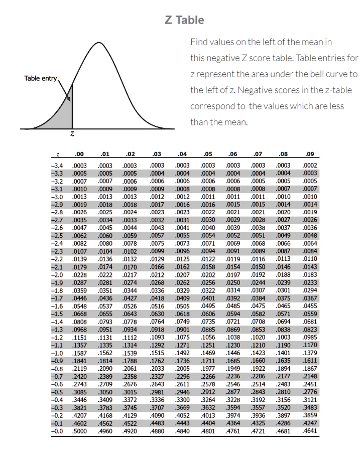
\(z\)-scores come from what is called a standard normal distribution, which is just a normal distribution with a mean of 0 and standard deviation (and variance) of 1, or \(N(0, 1)\). We know a lot about the standard normal distribution. For example, we know the probability that a random draw from a normal distribution is greater than some number, less than some number, or between two numbers. In most statistics courses, this is where you’d be shown a \(z\)-score table. Rather than spending time on this table, here are some takeaways:
Let me add some words to all of this math. Remember, if we picked a random element out of a vector, we would expect that element to be \(\sigma\) units away from the mean. What is the \(z\)-score doing? It is scaling the distance from some value \(y\) to the mean \(\mu\) by a measure of the average distance from the mean, \(\sigma\). Therefore, values of \(z\) that are greater in absolute value than 1 indicate that \(y\) is farther than the average element, and values less then one indicate \(y\) is closer than average. Being more than two times the average distance from the mean, for example, is pretty rare – there is only a 2.28% chance. A first important feature of \(z\)-scores is that they allow for the comparison of values from different distributions (e.g. SAT and ACT). A second important feature is that they allow us to calculate probabilities for every normal distribution, regardless of the mean, variance, and/or units.
R has some pre-built functions to work with normal distributions.
pnorm() gives \(P(Z < y)\) when lower.tail = TRUE. When lower.tail = FALSE, this gives \(P(Z > y)\)
pnorm(0, lower.tail = TRUE): 0.5pnorm(2, lower.tail = TRUE): 0.9772499.pnorm(2, lower.tail = FALSE): 0.0227501.qnorm() is the opposite of pnorm() in that it converts probabilities into \(z\)-scores.
qnorm(0.9772499, lower.tail = TRUE): 2.0000006rnorm() generates random draws from a standard normal distribution with a given mean and standard deviation. The default mean is 0 and the default standard deviation is 1. In the next lecture, you will use a function called sample() that also generates random data, but by drawing from values you already have.