Regressions in R
Alexander Cardazzi
Quarantine, 2020
Setting Up R for Use
When you open up a blank RScript, there are a few things you may want to put at the very top of your code. I like to lead with any libraries I will need. While there are a lot of things you can do with base R, people write packages to make our lives easier. For example, here is a list of a few packages I use in almost all of my scripts:
lubridate: this package is for working with date objects. Dates are not always easy to work with but I cannot recommend this package enough. Cheatsheet.stargazer: this package makes regression output beautiful and simple. Cheatsheet.data.table: this is for reading in large CSVs.1scales: this is for changing the opacity of plot colors. Purely aesthetic, but I love it.
Note that before you load a library (library("scales")), you need to install the library (install.packages("scales")). Installing packages only has to be done the very first time you use a package, then it will be on your machine forever.
Next, I try to always set up a working directory. Suppose you have a folder for your project, and lets say that file path is: C:/Users/alexc/Dropbox/sharkAttacks. Within this folder, I might have subfolders like raw_data, cleaned_data, literature, code, etc. It is likely that I’ll want to save my script in the code folder but read/write data to the raw_data/cleaned_data folders. To make this simple, I can do this:
setwd("C:/Users/alexc/Dropbox/sharkAttacks/")
#read in data

# do stuff ...

setwd("../cleaned_data")
#write out data
This allows for more “flexible” code since we only specify the filepath once. Notice how I used “../cleaned_data” in the second setwd(). These two dots mean “go back one level”. This tells the computer to back out of the raw_data folder and go inside the cleaned_data folder. If you are unsure of your working directory, you can use getwd() to see what R is currently using.
The last thing is to read in the datasets you need. Suppose we are looking at auction data. We may have one file that has four columns: bid amount, a timestamp, item ID and bidder ID. Then, we might have another file with information about each item, like retail price, country of origin, etc. and a file with information about the bidders like age, experience, wealth, etc. I made up some data and threw it into some CSVs. The header of my script should look like this:
#library("enter library here")

setwd("C:/Users/alexc/Desktop/Empirical Workshop/data/bidding data")
rm(list = ls()) #this clears my workspace ... be careful with this

bidz <- read.csv("bids.csv", stringsAsFactors = FALSE)
itemz <- read.csv("items.csv", stringsAsFactors = FALSE)
ppl <- read.csv("bidders.csv", stringsAsFactors = FALSE)
You can check out the data by clicking on the object in the Enviornment tab, or typing View(bidz) into the console. Before we get too much farther, we need to explore the data. Here is a list of some invaluable functions. Mastering these few functions take you from level 1 to level 2, and can save you hours of time.
table()aggregate()match()
First, in the bidz data frame, we might want to see how many bids each item got. We can easily do this by calling:
table(bidz$itemID)##
## 16302 39820 45991
## 5 4 7Instead, maybe we care about the number of bids per item, per person. This is easily done by just adding a second argument to the function.
table(bidz$itemID, bidz$bidderID)##
## a b c j
## 16302 1 0 1 3
## 39820 1 1 2 0
## 45991 3 0 3 1Now that we have an idea of how many bids there are and where they are located, we may want to know the average bid. However, since things at an auction can be vastly different prices, we might want to find the average by some identifier. In this case, we want the average big per item.
aggregate(bidz$bid, by = list(bidz$itemID), FUN = mean)## Group.1 x
## 1 16302 5.6
## 2 39820 127.5
## 3 45991 45.0Instead, maybe we want to observe a rough estimate of revealed preferences. How much does each person value each item? Let’s take the max of the bids per item per person. There is an important nuance to note with this, however. While table() reports zero values (for example, person b did not bet on item 16302 thus the frequency of this is zero), aggregate is unable to do this. In our case of revealed preferences, one might infer a value of 0 given someone never bidding on an item.
aggregate(bidz$bid, by = list(bidz$itemID, bidz$bidderID), FUN = max)## Group.1 Group.2 x
## 1 16302 a 6
## 2 39820 a 140
## 3 45991 a 70
## 4 39820 b 100
## 5 16302 c 4
## 6 39820 c 150
## 7 45991 c 75
## 8 16302 j 10
## 9 45991 j 20What if we want to pull information from another dataset into the bids dataset? For example, what if we want to look at retail price minus bid price for each bid? We need to pull in the retail price from the itemz table. To do this, we need to match the itemIDs, and get the retail price where these match.
bidz$itemID; itemz$itemID## [1] 45991 45991 45991 45991 45991 45991 45991 16302 16302 16302 16302
## [12] 16302 39820 39820 39820 39820## [1] 45991 89001 65420 98610 87098 16302 39820 10020match(bidz$itemID, itemz$itemID) #this gives the location of each element of bidz$id in itemz$itemID## [1] 1 1 1 1 1 1 1 6 6 6 6 6 7 7 7 7itemz$retail[match(bidz$itemID, itemz$itemID)] #reorder the itemz$retail vector to associate with the matching of bidz$id into itemz$itemID## [1] 50 50 50 50 50 50 50 5 5 5 5 5 150 150 150 150bidz$diff <- itemz$retail[match(bidz$itemID, itemz$itemID)] - bidz$bid #subtraction
bidz[,c("itemID", "bid", "diff")] #print these three columns## itemID bid diff
## 1 45991 10 40
## 2 45991 20 30
## 3 45991 30 20
## 4 45991 50 0
## 5 45991 60 -10
## 6 45991 70 -20
## 7 45991 75 -25
## 8 16302 3 2
## 9 16302 4 1
## 10 16302 5 0
## 11 16302 6 -1
## 12 16302 10 -5
## 13 39820 100 50
## 14 39820 120 30
## 15 39820 140 10
## 16 39820 150 0These are some really important things in R. I would encourage you to go over this a few times and really understand what is going on. The power of these three functions cannot be overstated.
Plotting
One of the main selling points of R is its extremely powerful graphical capabilities. People online love to use a library called ggplot2, but I prefer using base R plotting. I say this as it might be of interest for you to look into that package. You can check out all the possible arguments for plot(), our workhorse, by using the help function, but here are some of the main, most important ones:
- type: “l” = line, “p” = point, “b” = both, “h” = histogram
- col: Color argument. 8 pages of colors here
- pch: Point type. I use 19 for solid dots, 4 for an ‘x’ and more here
- cex: Point size. I usually just use 1.
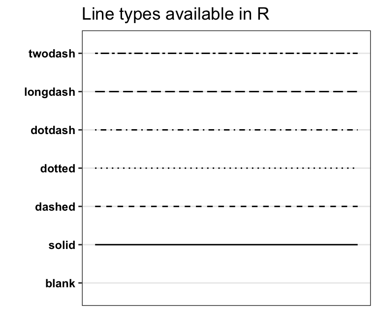
- lty: Line tpye. I use 1 for solid lines, 2 for dashed lines, and more here
- lwd: Line width. I usually use 1.
- main: this is to specify the title of the plot
- xlab / ylab: x/y labels
- xlim / ylim: x/y limits. Needs to be in c(min, max) format.
After a plot, you can also things using the following functions. Use the help function to learn more about these.
abline(): add a straight linepoints(): add points from datalines(): add lines from datalegend(): add a legend to the plotsegments(): add line segments
Let’s start by plotting bid against diff. Next, let’s add a horizontal line at zero and a vertical line at 50 (both arbitrary choices) and color them blue and red, respectively. Finally, let’s add a y = 50 - x line to the plot as well.
plot(bidz$bid, bidz$diff)

abline(h = 0, v = 50, col = c("blue", "red"))
abline(a = 50, b = -1) #y = a + bx
We can also make use of the bid order column in the bidz data if we want to make a time series type plot. On top of this, we can also change the background color and the number of plots displayed with the par() command. Just make sure to reset it after! For example:
par(bg = "pink", mfrow = c(1,3))

plot(bidz$bid, bidz$diff, col = "blue")
plot(bidz$time, bidz$bid, col = "dark green", pch = 4, cex = 2, xlab = "Time", ylab = "Bid ($)")
plot(bidz$time, bidz$diff, col = "red", pch = 19, main = "Diff vs Time", ylab = "", xlab = "")
par(bg = "white", mfrow = c(1,1))We can also conditionally color parts of the plot. We will go into these conditions more later, but the idea is to color the positive difference values dark green and the negative ones red.
plot(bidz$bid, bidz$diff, col = ifelse(bidz$diff >= 0, "dark green", "red"), pch = 19)
We can also plot distributions by either plot(table()) or hist(). The latter of these two options bins the data in a histogram format while the former will take a more exact approach.
par(mfrow = c(1,2))
plot(table(bidz$diff))
hist(bidz$diff)
par(mfrow = c(1,1))Using the scales package, we can change the opacity of the points, so we can see the concentration. I am going to make a 10000 random numbers and plot them against another 10000 numbers. The opacity will allow us to see overlaps.
library("scales")
set.seed(123)
plot(round(rnorm(10000),2), round(rnorm(10000),2),
     xlim = c(-1,1), ylim = c(-1,1),
     pch = 19,
     xlab = "", ylab = "", main = "",
     col = alpha("black", .2))
Econometrics
Let’s create a dataset right here and run some analyses. It is helpful to simulate data so we can know the exact parameters we are trying to estimate. I am going to create 5000 cars that can take on 3 possible colors, 20 possible ages, a maximum speed, a miles per gallon measurement (mpg), an indicator for ecofriendly, and a price. Speed and mpg are going to be functions of age, and eco friendly is going to be a 1 if a car is both faster than average AND has a higher mpg than average. This is to force some multicolinearity, heteroskedasticity and real-life-ness into the model.
N <- 5000
carz <- data.frame(color = sample(c("orange", "blue", "dark green"), N, replace = TRUE),
                   state = sample(c("NY", "NJ", "CT", "PA"), N, replace = TRUE),
                   age = sample(1:20, N, replace = TRUE),
                   maxSpeed = NA,
                   mpg = NA,
                   price = NA,
                   ecoFriendly = NA)
carz$color <- as.character(carz$color)
carz$maxSpeed <- rnorm(120 - (carz$age)/2, 8 + (carz$age)/4)
carz$mpg <- rnorm(20 - (carz$age)/10, 4 + (carz$age)/10)
carz$ecoFriendly <- round(ifelse(carz$mpg > mean(carz$mpg) & carz$maxSpeed > mean(carz$maxSpeed), .3, 0) + runif(N, 0, .7), 0)
carz$price <- ifelse(carz$color == "orange", 60, ifelse(carz$color == "blue", 30, 0)) - (5*carz$age) + (10*carz$maxSpeed) + (carz$mpg) + rnorm(N, 0, 5)
head(carz)
## color state age maxSpeed mpg price ecoFriendly
## 1 orange CT 5 8.079911 4.104663 122.31641 0
## 2 dark green NY 9 10.276107 4.509264 65.87716 0
## 3 blue CT 3 10.300084 3.750323 119.21220 1
## 4 blue NJ 10 12.523023 5.431819 110.33850 0
## 5 orange CT 15 10.390150 6.352688 101.76480 0
## 6 blue NJ 19 13.372110 5.231305 72.85922 0We can see the head of our data. Some plots might be in order to discover some underlying patterns.
par(mfrow = c(1,3))
plot(carz$maxSpeed, carz$price, col = carz$color)
abline(lm(carz$price ~ carz$maxSpeed))
plot(carz$age, carz$price, col = carz$color)
abline(lm(carz$price ~ carz$age))
plot(carz$mpg, carz$price, col = carz$color)
abline(lm(carz$price ~ carz$mpg))
From these plots, we can see that orange cars appear to constantly be selling for more, which is set in our price equation. If max speed is our variable of interest, maybe we want to consolidate these plots by findng the average price per max speed, rounded to the nearest decimal. We can also plot this by color as well.
par(mfrow = c(1,1))
plot(aggregate(carz$price, list(round(carz$maxSpeed, 1)), FUN = mean), ylab = "Price", xlab = "Max Speed", type = "p", pch = 19)
k <- aggregate(carz$price, list(round(carz$maxSpeed, 1), carz$color), FUN = mean)
plot(k$Group.1, k$x, ylab = "Price", xlab = "Max Speed", col = "white")
points(k$Group.1[k$Group.2 == "orange"], k$x[k$Group.2 == "orange"], col = "orange", pch = 19)
points(k$Group.1[k$Group.2 == "blue"], k$x[k$Group.2 == "blue"], col = "blue", pch = 19)
points(k$Group.1[k$Group.2 == "dark green"], k$x[k$Group.2 == "dark green"], col = "dark green", pch = 19)
Summary Stats
To create summary statistics of our dataset, we can use the stargazer(). When a data frame is passed to stargazer, it automatically makes summary stats for all numeric variables.
library("stargazer")##
## Please cite as:## Hlavac, Marek (2018). stargazer: Well-Formatted Regression and Summary Statistics Tables.## R package version 5.2.2. https://CRAN.R-project.org/package=stargazerstargazer(carz, type = "text")##
## ==================================================================
## Statistic N Mean St. Dev. Min Pctl(25) Pctl(75) Max
## ------------------------------------------------------------------
## age 5,000 10.454 5.803 1 5 16 20
## maxSpeed 5,000 10.624 1.755 5.379 9.313 11.919 15.385
## mpg 5,000 5.038 1.157 1.217 4.256 5.831 9.183
## price 5,000 89.030 30.310 12.562 66.176 112.032 172.718
## ecoFriendly 5,000 0.439 0.496 0 0 1 1
## ------------------------------------------------------------------Regressions
Suppose we are given this dataset and we are tasked with deriving a model for price, and a model for predicting if a car is ecofriendly. First, let’s attempt to model price with the lm() function, and then with the felm() function.
lm()
Let’s write down an econometric model like the one below. This is what we will estimate.
\[ P_i = \alpha_c + \beta Age_i + \gamma MPG_i + \delta Speed_i + \epsilon_i \]
reg1 <- lm(price ~ age, data = carz)
reg2 <- lm(price ~ age + mpg + maxSpeed, data = carz)
reg3 <- lm(price ~ age + mpg + maxSpeed + color, data = carz)
reg4 <- lm(price ~ age + mpg + maxSpeed + color + state, data = carz)
stargazer(reg1, reg2, reg3, reg4,
          type = "text",
          add.lines = list(c("Color FE", "N", "N", "Y", "Y"),
                           c("Robust SE", "N", "N", "N", "N")),
          omit = "color", omit.stat = "f",
          covariate.labels = c("Age in Years", "Miles Per Gallon", "Max. Speed"))
##
## =============================================================================================
## Dependent variable:
## -------------------------------------------------------------------------
## price
## (1) (2) (3) (4)
## ---------------------------------------------------------------------------------------------
## Age in Years -2.500*** -5.012*** -5.035*** -5.035***
## (0.065) (0.113) (0.023) (0.023)
##
## Miles Per Gallon 0.661* 0.869*** 0.868***
## (0.350) (0.070) (0.070)
##
## Max. Speed 9.777*** 10.018*** 10.016***
## (0.356) (0.072) (0.072)
##
## stateNJ -0.382*
## (0.202)
##
## stateNY -0.156
## (0.200)
##
## statePA -0.390*
## (0.200)
##
## Constant 115.163*** 34.224*** 30.731*** 30.997***
## (0.776) (3.246) (0.661) (0.674)
##
## ---------------------------------------------------------------------------------------------
## Color FE N N Y Y
## Robust SE N N N N
## Observations 5,000 5,000 5,000 5,000
## R2 0.229 0.331 0.973 0.973
## Adjusted R2 0.229 0.330 0.973 0.973
## Residual Std. Error 26.616 (df = 4998) 24.805 (df = 4996) 4.984 (df = 4994) 4.983 (df = 4991)
## =============================================================================================
## Note: *p<0.1; **p<0.05; ***p<0.01We now have estimates for each of parameters outlined in the written out model. Let’s suppose that for some reason, you think there is an issue with data from a certain state due to some funky regulations. Perhaps this regulation only affects old cars in that state. We can limit our dataset, instead of dropping observations, by using the following code.
lim <- carz$state %in% c("NY", "PA", "CT") #or, carz$state != "NJ"
reg1a <- lm(price ~ age, data = carz[lim,])

lim <- !(carz$state == "NJ" & carz$age > 15)
reg1b <- lm(price ~ age, data = carz[lim,])
felm()
In this sample of data, we do not have many fixed effects. However, there may be cases where there can be hundreds or even thousands. To handle this, the felm() function is very handy. This will partial out the fixed effects and hide them from the output. Further, it also has the ability to do instrumental variables and clustered standard errors. The structure of the arguments of felm() are as follows: felm(y ~ x1 + x2 | FE | x1 ~ z | CLSE, data = dataset). The first section is the formula without fixed effects, followed by fixed effects, followed by the formula for the IV, followed by the variable for clustering the standard errors. One thing to be careful about is multicolinearity. felm() will spit out a warning/error if a variable in the regular formula is perfectly colinear with the fixed effects. For example, if one variable is binary and tells if the observation comes from a democratic state but you’ve also included state fixed effects, there will be a warning/error.
In this setting, we can estimate both the regular standard errors as well as robust standard errors. I am not advocating for using color as an appropriate cluster, but rather just using it as an example.
library("lfe")## Loading required package: Matrixlibrary("sandwich")
library("lmtest")## Loading required package: zoo##
## Attaching package: 'zoo'## The following objects are masked from 'package:base':
##
## as.Date, as.Date.numeric##
## Attaching package: 'lmtest'## The following object is masked from 'package:lfe':
##
## waldtestreg51 <- lm(price ~ age + mpg + maxSpeed + color, data = carz)
reg52 <- felm(price ~ age + mpg + maxSpeed | color | 0 | 0, data = carz)
reg61 <- felm(price ~ age + mpg + maxSpeed | color | 0 | color, data = carz)
reg62 <- lm(price ~ age + mpg + maxSpeed + color, data = carz)
reg62 <- coeftest(reg62, vcovCL, cluster = carz$color) #reg62 <- coeftest(reg62, vcovHC) #this is for heteroskedasticity robust SE
stargazer(reg51, reg52,
reg61, reg62,
type = "text",
add.lines = list(c("Color FE", rep("Y", 4)),
c("Robust SE", "N", "N", "Y", "Y")),
omit = c("color", "Constant"), omit.stat = c("f", "ser"),
covariate.labels = c("Age in Years", "Miles Per Gallon", "Max. Speed"))##
## ==========================================================
## Dependent variable:
## -----------------------------------------
## price
## OLS felm coefficient
## test
## (1) (2) (3) (4)
## ----------------------------------------------------------
## Age in Years -5.035*** -5.035*** -5.035*** -5.035***
## (0.023) (0.023) (0.045) (0.045)
##
## Miles Per Gallon 0.869*** 0.869*** 0.869*** 0.869***
## (0.070) (0.070) (0.085) (0.085)
##
## Max. Speed 10.018*** 10.018*** 10.018*** 10.018***
## (0.072) (0.072) (0.107) (0.107)
##
## ----------------------------------------------------------
## Color FE Y Y Y Y
## Robust SE N N Y Y
## Observations 5,000 5,000 5,000
## R2 0.973 0.973 0.973
## Adjusted R2 0.973 0.973 0.973
## ==========================================================
## Note: *p<0.1; **p<0.05; ***p<0.01glm()
Maybe our variable of interest is predicting a binary outcome - whether or not a vehicle is eco-friendly. Instead of using just single standalone variables, we can also include interaction effects. Here is a short and intuitive explination of interactions.
reg1 <- glm(ecoFriendly ~ age, data = carz, family="binomial")
reg2 <- glm(ecoFriendly ~ age + mpg + maxSpeed, data = carz, family="binomial")
reg3 <- glm(ecoFriendly ~ age + mpg + maxSpeed + color, data = carz, family="binomial")
reg4 <- glm(ecoFriendly ~ age + mpg*maxSpeed + color, data = carz, family="binomial")

#create vectors, > mean
carz$mpg_high <- carz$mpg >= mean(carz$mpg)
carz$maxSpeed_high <- carz$maxSpeed >= mean(carz$maxSpeed)

reg5 <- glm(ecoFriendly ~ age + mpg_high*maxSpeed_high + color, data = carz, family="binomial")

stargazer(reg1, reg2, reg3, reg4, reg5,
          type = "text",
          add.lines = list(c("Color FE", "N", "N", "Y", "Y", "Y"),
                           c("Robust SE", "N", "N", "N", "N", "N")),
          omit = "color", #omit.stat = "f",
          covariate.labels = c("Age in Years", "Miles Per Gallon", "Max. Speed", "MPG > mean", "Max. Speed > mean"))
##
## =================================================================================
## Dependent variable:
## ------------------------------------------------------
## ecoFriendly
## (1) (2) (3) (4) (5)
## ---------------------------------------------------------------------------------
## Age in Years 0.082*** 0.008 0.008 0.007 -0.010
## (0.005) (0.009) (0.009) (0.010) (0.008)
##
## Miles Per Gallon 0.328*** 0.329*** -1.339***
## (0.030) (0.030) (0.176)
##
## Max. Speed 0.178*** 0.177*** -0.615***
## (0.030) (0.030) (0.087)
##
## MPG > mean 0.075
## (0.093)
##
## Max. Speed > mean -0.003
## (0.114)
##
## mpg:maxSpeed 0.158***
## (0.017)
##
## mpg_highTRUE:maxSpeed_high 1.809***
## (0.130)
##
## Constant -1.122*** -3.891*** -3.951*** 4.304*** -0.831***
## (0.063) (0.286) (0.290) (0.891) (0.083)
##
## ---------------------------------------------------------------------------------
## Color FE N N Y Y Y
## Robust SE N N N N N
## Observations 5,000 5,000 5,000 5,000 5,000
## Log Likelihood -3,294.039 -3,216.537 -3,214.722 -3,167.872 -3,026.408
## Akaike Inf. Crit. 6,592.078 6,441.073 6,441.445 6,349.744 6,066.815
## =================================================================================
## Note: *p<0.1; **p<0.05; ***p<0.01Differences in Differences
With a lot of focus in economics being on causal inference, it is important to be exposed to these things and learn to program them. I am not going to try to explain Differences in Differences here, but you can take a look at this code and check out what’s happening analytically and graphically.
library("scales")
set.seed(321)
data.frame(state = c(rep("NY", 40), rep("NJ", 40), rep("CT", 40), rep("PA", 40)),
           year = rep(c(1960:1999), 4),
           x1 = c(rnorm(40, 0, 1), rnorm(40, 0, 2), rnorm(40, 4, 1), rnorm(40, 4, 2)),
           x2 = c(rnorm(40, 6, 1), rnorm(40, 2, 1), rnorm(40, 3, 2), rnorm(40, 7, 1)),
           treat = c(rep(1, 40), rep(0, 120)),
           post = c(rep(c(rep(0, 25), rep(1, 15)), 4))) -> did

did$y <- -did$x1 + 4*did$x2 + 3*did$treat + 2*did$post + 5*did$treat*did$post + rnorm(160, 0, 2)
plot(did$year, did$y, col = "white", main  = "", ylab = "Y", xlab = "Year")
lines(did$year[did$state == "NY"], did$y[did$state == "NY"], col = alpha("orange", .25), lwd = 3)
lines(did$year[did$state == "NJ"], did$y[did$state == "NJ"], col = alpha("dark green", .25), lwd = 3)
lines(did$year[did$state == "CT"], did$y[did$state == "CT"], col = alpha("dark green", .25), lwd = 3)
lines(did$year[did$state == "PA"], did$y[did$state == "PA"], col = alpha("dark green", .25), lwd = 3)
abline(v = 1985)

segments(x0 = c(rep(1960, 2), rep(1985, 2)),
         x1 = c(rep(1985, 2), rep(1999, 2)),
         y0 = c(mean(did$y[did$treat == 1 & did$post == 0]),
                mean(did$y[did$treat == 0 & did$post == 0]),
                mean(did$y[did$treat == 1 & did$post == 1]),
                mean(did$y[did$treat == 0 & did$post == 1])),
         y1 = c(mean(did$y[did$treat == 1 & did$post == 0]),
                mean(did$y[did$treat == 0 & did$post == 0]),
                mean(did$y[did$treat == 1 & did$post == 1]),
                mean(did$y[did$treat == 0 & did$post == 1])),
         col = c("orange", "dark green", "orange", "dark green"),
         lwd = 4 ,lty = c(2, 3))
par(mfrow = c(1,3))
plot(did$year, did$y, col = "white", main  = "", ylab = "Y", xlab = "Year")
segments(x0 = c(rep(1960, 2), rep(1985, 2)),
         x1 = c(rep(1985, 2), rep(1999, 2)),
         y0 = c(mean(did$y[did$treat == 1 & did$post == 0]),
                mean(did$y[did$treat == 0 & did$post == 0]),
                mean(did$y[did$treat == 1 & did$post == 1]),
                mean(did$y[did$treat == 0 & did$post == 1])),
         y1 = c(mean(did$y[did$treat == 1 & did$post == 0]),
                mean(did$y[did$treat == 0 & did$post == 0]),
                mean(did$y[did$treat == 1 & did$post == 1]),
                mean(did$y[did$treat == 0 & did$post == 1])),
         col = alpha(c("orange", "dark green", "orange", "dark green"), .4),
         lwd = 4 ,lty = c(2, 3))

plot(did$year, did$y, col = "white", main  = "", ylab = "Y", xlab = "Year")
diff1 <- mean(did$y[did$treat == 1 & did$post == 1]) - mean(did$y[did$treat == 1 & did$post == 0])
diff2 <- mean(did$y[did$treat == 0 & did$post == 1]) - mean(did$y[did$treat == 0 & did$post == 0])
segments(x0 = c(rep(1960, 2), rep(1985, 2)),
         x1 = c(rep(1985, 2), rep(1999, 2)),
         y0 = c(0,
                0,
                diff1,
                diff2),
         y1 = c(0,
                0,
                diff1,
                diff2),
         col = alpha(c("orange", "dark green", "orange", "dark green"), .4),
         lwd = 4 ,lty = c(2, 3))

plot(did$year, did$y, col = "white", main  = "", ylab = "Y", xlab = "Year")
segments(x0 = c(rep(1960, 2), rep(1985, 2)),
         x1 = c(rep(1985, 2), rep(1999, 2)),
         y0 = c(0,
                0,
                diff1 - diff2,
                0),
        y1 = c(0,
                0,
                diff1 - diff2,
                0),
         col = alpha(c("orange", "dark green", "orange", "dark green"), .4),
         lwd = 4,lty = c(2, 3))
segments(x0 = 1985, y0 = 0, y1 = diff1-diff2, col = "red", lwd = 3)
print(diff1-diff2)## [1] 5.254047stargazer(lm(y ~ x1 + x2 + treat*post, data = did), type = "text", omit.stat = c("f", "ser"), omit = c("x", "Constant"))##
## ========================================
## Dependent variable:
## ---------------------------
## y
## ----------------------------------------
## treat 2.383***
## (0.533)
##
## post 1.972***
## (0.370)
##
## treat:post 5.679***
## (0.739)
##
## ----------------------------------------
## Observations 160
## R2 0.968
## Adjusted R2 0.967
## ========================================
## Note: *p<0.1; **p<0.05; ***p<0.01look into readRDS and saveRDS. Essentially, this saves an R object to your file directory. This provides two benefits over a CSV: it is zipped so much smaller and R can read the data in way quicker than a CSV. Drawback is you cannot open with Excel or Notepad. Should be used for LARGE datasets.↩