# Regression Discontinuity
Alex Cardazzi
All materials can be found at
alexcardazzi.github.io.
## Regression Discontinuity
In this final module, we will discuss Regression Discontinuity Design
(“RD” or “RDD”). As a bit of a peak behind the curtain, these modules
have been ordered from easiest to hardest (in my opinion) to find “in
the wild.” By this, I mean that it’s usually easier for people to come
up with a setting for DiD compared to IV, which may have become apparent
in the imagination exercises. Knowing this, you might consider RDD to be
the most difficult design to pull off. In some ways, this is true, but
the intuition behind RDD is fairly simple and the method is regarded by
many to be the most credible causal inference design (aside from an RCT,
of course).
### Flagship Universities
Let’s once again motivate this methodology with an example from a
published paper. Human capital accumulation, via educational attainment,
is an often studied determinant of labor market outcomes and quality of
life. Perhaps a more interesting question is the effect of school choice
on these same outcomes. In particular, what are the returns to attending
a state’s “flagship” university? In [a 2009 paper in *The Review of
Economics and Statistics*](https://www.jstor.org/stable/25651372), Mark
Hoekstra examines this very question. Reading through this paper as you
work through these notes might prove to be a useful exercise (and it’s
less than 10 pages).
For context, the “flagship university” in Virginia is UVA. Hoekstra’s
paper was published in 2009, three years after completing his PhD at
University of Florida. Since Hoekstra used actual college admissions
data from the examined flagship, we can make an educated guess at which
flagship university gave him the data.
To address the question of returns to attending the flagship, let’s
think through the other approaches we’ve learned thus far. First,
students are not randomly assigned to colleges and universities, so we
cannot simply estimate a model with an indicator for attending the
flagship like we would in an RCT. Second, this type of question would
not be a case study, so we can quickly rule out synthetic control.
Third, we could think about DiD or controlling for observable
characteristics. With the latter, we could look at the subset of
students admitted into the flagship university, and compare the outcomes
of those who attended the school to the outcomes of those who did not.
An issue with controlling for observables is that, conditional on
acceptance, there are likely some unobservable factors that causes both
student outcomes and the decision to attend the flagship.[^1] DiD also
presents a challenge due to a lack of a pre-period. Without
pre-treatment earnings, we cannot measure pre-post differences.
The most recent method we discussed, IV, would be an interesting way to
address this question. To do so, we would need some instrument that
causes college admission/attendance that is uncorrelated with earning
potentials. David Card, in 1993, used proximity to college as an
instrument for attending college and found positive returns to
schooling. In this paper, Card is estimating the extensive margin
(college vs no college). However, this does not really get at the
intensive margin: the returns to attending a relatively more selective
college (as proxied by flagship status).
Before getting into how Hoekstra addressed this question, we need to
understand the admission decision rule for the university. Each
student’s highschool GPA corresponds to a particular SAT score needed
for admission. For example, a student with a 3.0 might need a 1,000 SAT,
but a student with a 2.9 GPA might need a 1,100 SAT. Each student is
then awarded points based on how different their SAT was from the
required SAT. If the 2.9 student scored a 1,150 on their SAT, they would
be given 50 points. If the 3.0 student scored 1,150, they would be
awarded 150 points. Only students with non-negative amounts of points
were admitted into the university.
This “score” determines admission into the flagship, which would be the
treatment in this case. However, individuals barely to the right of the
cutoff are probably similar to those barely to the left. In fact, the
only difference between students with a score of -10 and +10 is a
question or two on the SAT. These students are practically the same, but
the small difference in their SAT scores earns one of them admission
into the flagship university.
In short, Hoekstra takes advantage of this setup by examining earning
outcomes for students right around this cutoff to estimate the causal
treatment effect of being admitted into the state’s flagship university.
Before getting into the nitty gritty, let’s define some terms.
- **Running Variable**: this is the measure that partially determines
treatment. In our example, the SAT score would be the running
variable.
- **Cutoff**: this is the *value* of the running variable that
determines treatment. Since the SAT scores have been adjusted to be
centered at zero, depending on the GPA, zero is the cutoff in the
example. As another example, when studying retirement, 65 would be a
cutoff value and age the running variable.
- **Bandwidth**: this is the maximum distance from the cutoff you are
willing to consider observations “similar”. You may be willing to
consider students $\pm 100$ points away from the cutoff similar, but
students $\pm 200$ points away from the cutoff less than comparable.
Both a continuous running variable and a clearly defined cutoff are
absolutely necessary to estimate regression discontinuity designs.
### Assumptions
Much like how IV requires excludability and validity, while DiD requires
parallel trends, there are two main assumptions in RDDs. These
assumptions ensure the treatment is plausibly exogenous, or effectively
randomly assigned.
First, individuals close to the cutoff should be similar in both their
observable and unobservable characteristics. In other words, the *only*
thing that changes at the cutoff is treatment, and individuals are
identical otherwise. In the case of SAT scores and admissions, a few
more correct (incorrect) questions on the SAT is hardly a meaningful
difference in terms of student quality. Formally, this is a
**continuity** assumption: the average potential outcomes,
$E[Y(0)]$ and $E[Y(1)]$, change smoothly as the running variable crosses
the cutoff, with no jump of their own. If so, any jump in the outcome at
the cutoff can only be due to the treatment.
Second, individuals may not manipulate their being on either side of the
cutoff. A violation of this assumption is a clear indication of
non-random treatment assignment. Typically, it’s best if the individuals
do not even know about the cutoff, because then manipulation is
impossible. In the case of admissions, the SAT cutoff was unknown to
students. If it were known, the students could have kept taking the SAT
until they got their desired score on the test for admission.
*If* both of these assumptions are met, RDD is often considered the best
you can do without having an RCT.
/
### Sharp RDD
Let’s suppose that being above the SAT threshold for your GPA
automatically guaranteed admission into the university. Further, once
admitted, students decided to enroll in the university 100% of the time.
While this is certainly unrealistic in this setting (since both students
and admissions offices have free will), this is the case for some
things, like government policies.
For example, during the pandemic, the government gave out stimulus
checks. If they decided to only give out stimulus checks to individuals
who made less than \$75,000 in 2019, this would fit the setting outlined
above. In this case, the running variable would be 2019 income, and the
cutoff would be \$75,000. People making \$77,000 are probably similar to
people making \$73,000. Also, since the stimulus checks were given out
based on (predetermined) pre-pandemic income, which side of the cutoff
people fall on is not manipulable.
If we wanted to estimate the effect of stimulus checks on some outcome
$Y$ in this setting, we could model it explicitly as follows:
$$Y = \beta_0 + \beta_1 (\text{Running - Cutoff}) + \beta_2 [(\text{Running - Cutoff})\times D] + \beta_3 D + \epsilon$$
where $D$ is equal to $1$ when the running variable takes on a value
greater than the cutoff.
$\beta_0$ represents the intercept, or the expectation of $Y$ when all
other variables are equal to zero. $\beta_1$ controls for the
relationship between the running variable and $Y$ *before* the cutoff,
whereas $\beta_2$ controls for the relationship between the running
variable and $Y$ *after* the cutoff. In other words, we are fitting two
different lines before and after the cutoff value. $\beta_3$ represents
the parameter of interest – the effect of moving from the not treated
group to the treated group. Of course, you may want other controls in
this model, but this would be the most basic set up.
The idea of including the centered running variable interacted with the
treatment variable is to control for potentially different relationships
between the running variable and the outcome on either side of the
cutoff. However, the direct interpretation of $\beta_2$ is the *change*
in the relationship when moving from one side of the cutoff to the
other. Therefore, to the effect of the running variable on the outcome
on the left of the cutoff is $\beta_1$. The effect of the running
variable on the outcome on the right of the cutoff is
$\beta_1 + \beta_2$.
Note that in this model, we are assuming a linear fit on either side of
the cutoff. In more modern applications, econometricians tend to use
more flexible (i.e. complicated) methods to estimate the relationships
on either side of the cutoff. We will demonstrate some of this in the
programming section of the notes, but it’s important to realize that
this linear approximation is mostly for instructional purposes. For
example, we could instead use a quadratic fit, or some other functional
form. Remember, our primary interest is estimating/interpreting the
change in the outcome at the cutoff. Therefore, how we estimate the pre-
and post- cutoff relationships between the running variable and outcome
is only important insofar that we can appropriately fit the data around
the cutoff. More on this later.
### Fuzzy RDD
Hoekstra’s paper about college admissions is a bit unlike the
hypothetical case regarding stimulus checks. Admission decisions are
influenced by GPA and SAT scores, but also extra curricular activities
and extraordinary circumstances. In addition, college students often get
admitted to more than one school, so the probability that an admitted
student enrolls in any given university is less than one. All of this is
to say that students below the cutoff may still enroll in the flagship
university, and students above the cutoff may choose to not enroll.
Therefore, being above or below the cutoff does not perfectly determine
treatment status, but it should still significantly increase the
probability of treatment.
This should sound a lot like an instrumental variable. Remember, being
drafted into the military did not perfectly determine military status,
but it did significantly influence the probability of enlistment. We are
going to treat the running variable and cutoff as an instrument in cases
like this. Therefore, we need a two-stage estimation procedure, just
like IV.
The first-stage would be to estimate treatment, or enrollment, via the
cutoff:
$$\text{Enroll} = \alpha_0 + \alpha_1 (\text{Running - Cutoff}) + \alpha_2 [(\text{Running - Cutoff})\times D] + \alpha_3 D + \epsilon$$
Once we gather the fitted values for enrollment ($\widehat{Enroll}$), we
can plug those values into the second stage as follows:
$$Y = \beta_0 + \beta_1 (\text{Running - Cutoff}) + \beta_2 [(\text{Running - Cutoff})\times D] + \beta_3 \widehat{\text{Enroll}} + \epsilon$$
Here, our parameter of interest is represented by $\beta_3$ once again.
Note that we still control for the pre- and post-cutoff relationships
between the running variable and the outcome. Of course, all of the
previous discussion about this being a linear fit still applies.
### RDD Is a Special Case of IV
Putting the pieces together, RDD is a special case of IV. In a fuzzy
design, the instrument is an indicator for being above the cutoff, and
the first and second stages are exactly the ones from the IV notes. In a
sharp design, being above the cutoff determines treatment perfectly, so
the instrument *is* the treatment. The first stage is a perfect fit, and
the two stages collapse into the single regression we wrote above. The
IV conditions have RDD counterparts as well. Relevance is the jump in
treatment at the cutoff. Excludability is the continuity assumption:
nothing else jumps at the cutoff, which is why we also check that
individuals are not manipulating the running variable.
### Bandwidth Selection
Regardless of whether we choose either a sharp or fuzzy design, it’s
important to consider the sample we use to estimate our treatment
effect. Specifically, there’s still the question of bandwidth. Choosing
a too-large bandwidth will increase the sample size (thus the
statistical power and/or precision) but also increases the risk of bias.
The additional observations that get let in towards the edges of the
bandwidth are less likely to be similar and could introduce confounding.
On the other hand, choosing a too-small bandwidth will reduce the risk
of bias, but also reduce the sample size and thus accuracy of the
estimates.
There are many different ways to select a bandwidth, though we will
eventually have R do this for us. However, the most intuitive approach
to selecting a bandwidth is simply choosing something “reasonable” with
respect to the empirical setting. Then, we can vary the bandwidth to
test the sensitivity of the estimate to our choice of bandwidth. In
applications, this can be done by continually re-estimating the model
inside of a `for` loop and collecting the results.
The figures above are taken from NHK’s textbook chapter and demonstrate
the effects of bandwidth choice. In the figure to the left, no bandwidth
is used, and thus all of the observations are included in the
estimation. This figure also demonstrates the consequences of using only
linear fits. The treatment effect would be the vertical distance between
the two solid lines at the cutoff value. In this figure, the treatment
is clearly exaggerated by the poor fit of the linear model.
In the figure to the right, the fit of the linear model is improved by
the use of a bandwidth. Even though the data clearly exhibit a
non-linear relationship over the domain of the running variable, linear
approximations work just fine right around the cutoff.
In the above series of figures, NHK ditches the bandwidth in favor of
more flexible functional forms. In the first panel, NHK uses a quadratic
fit on either side of the cutoff, and the treatment effect looks similar
to that of the linear fit with a bandwidth. In the second panel, he uses
an order-6 polynomial
(i.e. $\alpha_6x^6 + \alpha_5x^5 + ... + \alpha_1x + \alpha_0$) which
does a better job of fitting the data but does not really add much to
the estimation of the cutoff. In the third panel, he uses an order-25
polynomial which, at this point, *overfits* the data. In other words,
this model is picking up patterns that do not actually exist. The fourth
panel exists as a reference.
These figures provide visual evidence of ways to use either complicated
models or bandwidths to estimate RDDs. In practice, though, we will use
both simultaneously.
## Coding
In this section, we are going to analyze a pretend policy implemented by
ODU. Let’s suppose that on the first day of freshman year, every student
had to take a general college readiness exam. The purpose of this exam
is to identify students who might need some extra help as they begin
their college career. ODU then *forces* students to use a tutor if and
only if they score below a 70 on this exam. Students are then given a
second exam immediately before graduation to test how much they’ve
learned.
ODU has prompted us with measuring how much tutoring can improve test
scores. Since we observe treatment being determined by some rule, we can
explore using RDD. There are four steps we need to take:
1. Determine if our RDD is sharp or fuzzy.
2. Check for manipulation around the cutoff.
3. Check for a discontinuity at the cutoff in the outcome.
4. Estimate the discontinuity.
The figures below demonstrate these four steps.
### Sharp vs Fuzzy
First, we need to determine whether our RDD is sharp or fuzzy. Remember,
if the cutoff determines treatment *with certainty*, then we should use
a sharp RDD. Otherwise, fuzzy is the way to go.
In the following chunk below, I have written a function to simulate data
that matches with our make-believe setting. Notice that the function
accepts three arguments: sample size (`N`), a cutoff exam score
(`CUTOFF`), and the probability of treatment for those above the cutoff
(`PROB`).
``` r
genr_data <- function(N = 1000, CUTOFF = 70, PROB = 1){
df <- data.frame(id = 1:N,
exam1 = rbeta(N, 7, 2),
exam2 = rbeta(N, 5, 3),
tutor = NA)
df$exam1 <- round(df$exam1 * 100)
df$tutor <- ifelse(df$exam1 < CUTOFF,
sample(c(0, 1), N, replace = T,
prob = c(1 - PROB, PROB)),
sample(c(0, 1), N, replace = T,
prob = c(PROB, 1 - PROB)))
df$exam2 <- round((df$exam2 * 40) + (10 * df$tutor) + (df$exam1 / 2))
return(df)
}
```
``` r
genr_data <- function(N = 1000, CUTOFF = 70, PROB = 1){
df <- data.frame(id = 1:N,
exam1 = rbeta(N, 7, 2),
exam2 = rbeta(N, 5, 3),
tutor = NA)
df$exam1 <- round(df$exam1 * 100)
df$tutor <- ifelse(df$exam1 < CUTOFF,
sample(c(0, 1), N, replace = T,
prob = c(1 - PROB, PROB)),
sample(c(0, 1), N, replace = T,
prob = c(PROB, 1 - PROB)))
df$exam2 <- round((df$exam2 * 40) + (10 * df$tutor) + (df$exam1 / 2))
return(df)
}
```
Since ODU enforces tutoring for *all* students who scored below a 70 in
this hypothetical case, we would conclude this to be a sharp regression
discontinuity. If tutoring was instead available to all, but only
suggested/advertised to students who scored below 70 on their exam, this
would be a fuzzy regression discontinuity.
## Sharp vs Fuzzy
Let’s use this function to generate data using the default argument
values.
The default arguments generate data consistent with a sharp regression
discontinuity since `PROB` is set to 1. If this were a number between 0
and 1, the data would be consistent with a fuzzy design.
``` r
# You may change the parameters in the function below.
df <- genr_data()
head(df)
```
### Cutoff Manipulation
Next, we need to check the assumption that individuals are not
manipulating their being on a specific side of the cutoff. There are
formal statistical tests for this, but the intuition is simple. If the
distribution along the running variable appears continuous at the
cutoff, then our assumption holds. If there is manipulation, we should
see a distribution mass on one side of the cutoff. We need to check the
distribution of the running variable as well as any other controls.
An example of a distribution that is *clearly* manipulated is the
distribution of marathon finishing times. See below for this
distribution.
Notice how running times appear to be fairly normally distributed.
However, within each distribution, there are huge spikes around each
hour. This is because runners target these times as benchmarks, and will
push themselves to finish before four hours rather than right after. If
we see something like this in our test score data, we would have a
violation of the manipulation assumption which could invalidate our RDD.
## Cutoff Manipulation
To start, let’s plot a histogram of scores from `exam1`.
``` r
# Plot distribution of exam1
plot(table())
abline(v = 69.5, col = "tomato")
```
Depending on the data that was generated, you might get a figure that
makes it look like there’s some manipulation going on. However, if you
increase the sample size of the generated data, this should eventually
wash away. What if we don’t have the luxury of simply increasing our
sample size? We need a statistical test to help us.
We are going to use a function from the `rddensity` package to help us
test for manipulation. The function has the same name as the package,
and we need to provide the running variable and the cutoff value. See
the code in the below chunk:
``` r
dens <- rddensity(df$exam1, c = 70)
summary(dens)
```
The output is verbose, but we should focus the line that says “Robust”.
This line contains a p-value that tests the difference in density at the
cutoff. You would interpret this p-value just as you would for a
regression coefficient. We can also create a visualization using the
`rdplotdensity()` function. To do this, we need to supply the result of
`rddensity()` and the running variable. See the following.
``` r
# Generate the distribution:
rdplotdensity(rdd = dens, X = df$exam1)
```
If our statistical test suggests that there is no manipulation, then we
can proceed with our analysis.
### Discontinuity
The penultimate step is to visually check for a discontinuity in the
outcome variable. To do this, generate a plot where the running variable
is on the x-axis and the outcome is on the y-axis. Note that in some
cases, you can use a simple scatter plot. However, with a lot of data,
you might want to use aggregate to make the figure more concise.
``` r
# Generate a scatterplot below
# Put the running variable on the x-axis
# and the outcome on the y-axis
# You might need to use alpha() for transparency
plot(, pch = 19)
abline(v = 69.5, col = "tomato")
```
``` r
# Next, use aggregate() before plotting
agg <- aggregate(list(outcome = ),
list(running = ),
mean)
plot(agg$running, agg$outcome, pch = 19)
abline(v = 69.5, col = "tomato")
```
Note that while we want to see a discontinuity in the outcome variable,
we *do not* want to see any discontinuities in any other observable
variables, as this suggests evidence of confounding and/or manipulation
at the cutoff.
### Estimation
Finally, we can estimate the treatment effect, which is the change in
the outcome variable right at the cutoff value. To illustrate, we will
first estimate the cutoff *parametrically* using a sharp design followed
by a fuzzy design. Next, we’ll use the `rdrobust` package to estimate
the discontinuity with *nonparametric* methods.
“Parametric” means that we are imposing a functional form onto the
model. For example, $Y = \alpha + \beta X$ is *parameterized* with a
slope and intercept. A nonparametric model is something that does not
have a particular functional form, and is therefore more flexible. Using
a parametric model trades off accuracy for interpretability. However, in
RDD, economists hardly ever interpret the relationship between the
running variable and the outcome, so they elect for accuracy.
Ultimately, this allows for a more accurate and interpretable estimate
of the treatment effect.
First, we need to create an additional variable to help us in the
estimation procedure. Specifically, we’ll create a centered running
variable. In other words, the running variable minus the cutoff. Once we
have this variable, we can estimate our RD. Remember, we are initially
estimating a sharp regression discontinuity. Our first model will
include the running variable and the tutor indicator. The assumption we
are making in doing this is that an additional point scored on the first
exam will have the same effect for students on either side of the
cutoff. Is this assumption reasonable? Probably, but it is an assumption
that we do not really need to make. Instead, we can interact the two
variables in the model, which will allow the relationship to change on
either side of the cutoff.
``` r
df$centered <- df$exam1 - 70
r1 <- lm(exam2 ~ centered + tutor, df)
r2 <- lm(exam2 ~ centered*tutor, df)
```
Table of Estimates
Code
``` r
r1 <- lm(exam2 ~ centered + tutor, df)
r2 <- lm(exam2 ~ centered*tutor, df)
library("modelsummary")
options(modelsummary_factory_default = 'tinytable')
options("modelsummary_format_numeric_latex" = "plain")
regz <- list(`(1)` = r1, `(2)` = r2)
coefz <- c("centered" = "Centered Exam 1 Score",
"tutor" = "Tutoring",
"centered:tutor" = "Centered Exam 1 Score x Tutoring",
"(Intercept)" = "Constant")
gofz <- c("nobs", "r.squared")
modelsummary(regz,
title = "Effect of Tutoring on Exam 2 Scores",
estimate = "{estimate}{stars}",
coef_map = coefz,
gof_map = gofz)
```
Output
+----------------------------------+-----------+-----------+
| | (1) | (2) |
+==================================+===========+===========+
| Centered Exam 1 Score | 0.539*** | 0.522*** |
+----------------------------------+-----------+-----------+
| | (0.027) | (0.032) |
+----------------------------------+-----------+-----------+
| Tutoring | 10.288*** | 10.493*** |
+----------------------------------+-----------+-----------+
| | (0.833) | (0.862) |
+----------------------------------+-----------+-----------+
| Centered Exam 1 Score x Tutoring | | 0.053 |
+----------------------------------+-----------+-----------+
| | | (0.057) |
+----------------------------------+-----------+-----------+
| Constant | 59.484*** | 59.711*** |
+----------------------------------+-----------+-----------+
| | (0.436) | (0.500) |
+----------------------------------+-----------+-----------+
| Num.Obs. | 1000 | 1000 |
+----------------------------------+-----------+-----------+
| R2 | 0.315 | 0.316 |
+----------------------------------+-----------+-----------+
Table: Effect of Tutoring on Exam 2 Scores
In the table, the first coefficient in the first column is an estimate
of the linear relationship between the student scores on exam 1 and the
scores on exam 2. The second estimate represents the effect of tutoring
on exam scores, which is our treatment effect.
These estimates were generated using a different instance of simulated
data, which might not match what you are working with in the WebR
chunks.
In the second column, the first estimate is the relationship between
exam 1 and exam 2 for students who did not get tutoring. In other words,
the relationship when exam 1 was above the cutoff. Therefore, the
relationship between exam 1 and exam 2 for students below the cutoff is
the sum of the first and third parameters. Interpreting these
coefficients is similar to interpreting interactions in a DiD setup.
Finally, the second estimate is, once again, our causal treatment
effect.
As a note before we move onto estimating a fuzzy design, we can also
apply bandwidths to our sample to eliminate observations that are far
from the cutoff. To apply a bandwidth, we can simply use the `subset`
argument in `lm()`. In particular, to keep only students who scored
within 10 points of the cutoff on the exam, we can use
`lm(..., subset = abs(df$centered) <= 10)`. Try this out in the previous
code chunk.
If this setting called for a fuzzy design, we would need to use being
above/below the cutoff as an instrument for whether the student took up
tutoring. In the code chunk below, I will demonstrate this mechanically
with `lm()` and then again with `feols()`. Remember, this is just an IV
set up!
``` r
df_fuzzy <- genr_data(PROB = 0.8)
df_fuzzy$centered <- df_fuzzy$exam1 - 70
df_fuzzy$above_cutoff <- ifelse(df_fuzzy$centered >= 0, 1, 0)
stage1 <- lm(tutor ~ centered + centered:above_cutoff
+ above_cutoff, df_fuzzy)
df_fuzzy$tutor_fitted <- stage1$fitted.values
stage2 <- lm(exam2 ~ centered + centered:above_cutoff
+ tutor_fitted, df_fuzzy)
summary(stage2)
cat("##### lm() above, feols() below ##### \n\n")
feols(exam2 ~ centered + centered:above_cutoff
| tutor ~ above_cutoff, df_fuzzy)
```
In the following, we will use `rdrobust()` from the package `rdrobust`.
Sometimes using packages can feel particularly like a black box, and I
am sympathetic to that feeling. It may be helpful to keep in the back of
your mind that the code below is simply performing a beefed up version
of the routines we used above.
To start, we will estimate a sharp regression discontinuity. See the
following for the code. We will provide the function with our outcome
and running variables as well as the cutoff value.
``` r
rd <- rdrobust(y = df$exam2, x = df$exam1, c = 70)
summary(rd)
```
Again, there is quite a bit of output from this function, so let’s break
it down. Most importantly, we have our treatment effect at the very
bottom under “Coef.” Note that in this specification, we get a negative
value. This because when moving in the positive direction along the
running variable, there is a jump down at the cutoff. We would still
interpret this as a positive effect of tutoring, because the treatment
is applied to those students on the left side of the cutoff. This
function also calculates p-values and confidence intervals for us so we
can make inference.
The second most important part is the bandwidth used to estimate this
effect. This is given by “BW est. (h)” towards the middle of the output.
As I mentioned earlier, this is chosen for us using data driven methods
that are outside the scope of these notes.
It’s often important to examine the treatment effect estimate’s
sensitivity to the choice of bandwidth. To address this, we can manually
vary the bandwidth by using the `h` argument in `rdrobust()`. A good way
to check is by halving and doubling the bandwidth and re-estimating the
model. Give this a try in the following chunk:
``` r
rd <- rdrobust(y = df$exam2, x = df$exam1, c = 70, h = )
summary(rd)
```
To turn this from a sharp RDD to a fuzzy design, we only need to make a
small tweak. Specifically, we would simply supply the treatment variable
inside the function: `fuzzy = df$tutor`. Try estimating a fuzzy RD using
function above again with data generated using `PROB = 0.8`.
Finally, one of the best parts of RDD studies are the aesthetically
pleasing, and particularly convincing, visualizations. We have already
shown some of this visualization above, but `rdrobust` provides us with
a helpful function.
``` r
# Visualize using rdplot
rdplot(y = df$exam2, x = df$exam1, c = 70,
# fuzzy = ,
x.label = "Running Variable",
y.label = "Outcome Variable",
title = "")
```
## Back to Flagships
RDD is relatively simple to estimate, convincing *and* intuitive. Again,
besides RCTs, this is the gold standard of causal inference research
designs. However, finding settings “in the wild” where one can use RDD
is often difficult and sometimes a matter of luck. So, before
concluding, let’s finish up our discussion of Hoekstra and flagship
universities.
Hoekstra uses a fuzzy regression discontinuity design because the cutoff
does not perfectly predict enrollment. However, he finds that the
probability of enrollment jumps up by almost 40 percentage points for
students immediately to the right of the SAT cutoff. So, it’s clear that
the cutoff plays a significant role in admission decisions. Hoekstra
also checks for manipulation at the cutoff but does not find any
evidence.
In the second part of the analysis, Hoekstra estimates the discontinuity
in the natural log of earnings for the students in the sample. After
applying the fuzzy RDD, he finds about a 13% increase in earnings due to
admission, and a 22% increase in earnings due to enrollment. Of course,
this raises questions about why/how this is. Unfortunately, Hoekstra is
unable to answer these questions given the data, but this certainly
opens up avenues for future research.
## NHK Videos
/
[^1]: In fact, some previous research has tried to mitigate these
concerns by using pairs of twins who choose to attend different
universities.
 In the above series of figures, NHK ditches the bandwidth in favor of
more flexible functional forms. In the first panel, NHK uses a quadratic
fit on either side of the cutoff, and the treatment effect looks similar
to that of the linear fit with a bandwidth. In the second panel, he uses
an order-6 polynomial
(i.e. $\alpha_6x^6 + \alpha_5x^5 + ... + \alpha_1x + \alpha_0$) which
does a better job of fitting the data but does not really add much to
the estimation of the cutoff. In the third panel, he uses an order-25
polynomial which, at this point, *overfits* the data. In other words,
this model is picking up patterns that do not actually exist. The fourth
panel exists as a reference.
These figures provide visual evidence of ways to use either complicated
models or bandwidths to estimate RDDs. In practice, though, we will use
both simultaneously.
 ### Sharp vs Fuzzy
First, we need to determine whether our RDD is sharp or fuzzy. Remember,
if the cutoff determines treatment *with certainty*, then we should use
a sharp RDD. Otherwise, fuzzy is the way to go.
In the following chunk below, I have written a function to simulate data
that matches with our make-believe setting. Notice that the function
accepts three arguments: sample size (`N`), a cutoff exam score
(`CUTOFF`), and the probability of treatment for those above the cutoff
(`PROB`).
``` r
genr_data <- function(N = 1000, CUTOFF = 70, PROB = 1){
df <- data.frame(id = 1:N,
exam1 = rbeta(N, 7, 2),
exam2 = rbeta(N, 5, 3),
tutor = NA)
df$exam1 <- round(df$exam1 * 100)
df$tutor <- ifelse(df$exam1 < CUTOFF,
sample(c(0, 1), N, replace = T,
prob = c(1 - PROB, PROB)),
sample(c(0, 1), N, replace = T,
prob = c(PROB, 1 - PROB)))
df$exam2 <- round((df$exam2 * 40) + (10 * df$tutor) + (df$exam1 / 2))
return(df)
}
```
``` r
genr_data <- function(N = 1000, CUTOFF = 70, PROB = 1){
df <- data.frame(id = 1:N,
exam1 = rbeta(N, 7, 2),
exam2 = rbeta(N, 5, 3),
tutor = NA)
df$exam1 <- round(df$exam1 * 100)
df$tutor <- ifelse(df$exam1 < CUTOFF,
sample(c(0, 1), N, replace = T,
prob = c(1 - PROB, PROB)),
sample(c(0, 1), N, replace = T,
prob = c(PROB, 1 - PROB)))
df$exam2 <- round((df$exam2 * 40) + (10 * df$tutor) + (df$exam1 / 2))
return(df)
}
```
Since ODU enforces tutoring for *all* students who scored below a 70 in
this hypothetical case, we would conclude this to be a sharp regression
discontinuity. If tutoring was instead available to all, but only
suggested/advertised to students who scored below 70 on their exam, this
would be a fuzzy regression discontinuity.
## Sharp vs Fuzzy
Let’s use this function to generate data using the default argument
values.
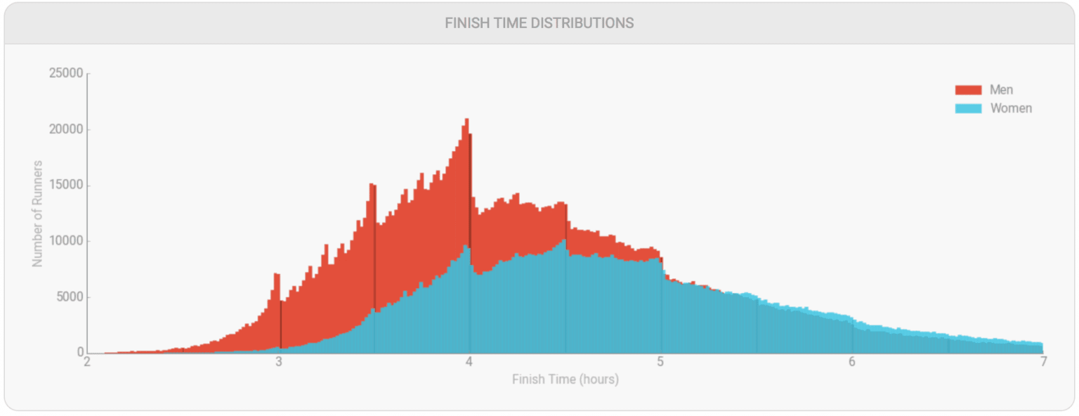 Notice how running times appear to be fairly normally distributed.
However, within each distribution, there are huge spikes around each
hour. This is because runners target these times as benchmarks, and will
push themselves to finish before four hours rather than right after. If
we see something like this in our test score data, we would have a
violation of the manipulation assumption which could invalidate our RDD.
## Cutoff Manipulation
To start, let’s plot a histogram of scores from `exam1`.
``` r
# Plot distribution of exam1
plot(table())
abline(v = 69.5, col = "tomato")
```
Depending on the data that was generated, you might get a figure that
makes it look like there’s some manipulation going on. However, if you
increase the sample size of the generated data, this should eventually
wash away. What if we don’t have the luxury of simply increasing our
sample size? We need a statistical test to help us.
We are going to use a function from the `rddensity` package to help us
test for manipulation. The function has the same name as the package,
and we need to provide the running variable and the cutoff value. See
the code in the below chunk:
``` r
dens <- rddensity(df$exam1, c = 70)
summary(dens)
```
The output is verbose, but we should focus the line that says “Robust”.
This line contains a p-value that tests the difference in density at the
cutoff. You would interpret this p-value just as you would for a
regression coefficient. We can also create a visualization using the
`rdplotdensity()` function. To do this, we need to supply the result of
`rddensity()` and the running variable. See the following.
``` r
# Generate the distribution:
rdplotdensity(rdd = dens, X = df$exam1)
```
If our statistical test suggests that there is no manipulation, then we
can proceed with our analysis.
### Discontinuity
The penultimate step is to visually check for a discontinuity in the
outcome variable. To do this, generate a plot where the running variable
is on the x-axis and the outcome is on the y-axis. Note that in some
cases, you can use a simple scatter plot. However, with a lot of data,
you might want to use aggregate to make the figure more concise.
``` r
# Generate a scatterplot below
# Put the running variable on the x-axis
# and the outcome on the y-axis
# You might need to use alpha() for transparency
plot(, pch = 19)
abline(v = 69.5, col = "tomato")
```
``` r
# Next, use aggregate() before plotting
agg <- aggregate(list(outcome = ),
list(running = ),
mean)
plot(agg$running, agg$outcome, pch = 19)
abline(v = 69.5, col = "tomato")
```
Note that while we want to see a discontinuity in the outcome variable,
we *do not* want to see any discontinuities in any other observable
variables, as this suggests evidence of confounding and/or manipulation
at the cutoff.
### Estimation
Finally, we can estimate the treatment effect, which is the change in
the outcome variable right at the cutoff value. To illustrate, we will
first estimate the cutoff *parametrically* using a sharp design followed
by a fuzzy design. Next, we’ll use the `rdrobust` package to estimate
the discontinuity with *nonparametric* methods.