# Introduction
Alex Cardazzi

All materials can be found at
<a href="https://alexcardazzi.github.io/econ708a.html"
target="_blank">alexcardazzi.github.io</a>.

## Introduction

Students enrolled in this class should have some pre-exposure to both
econometrics and R. This course is meant to move students from
estimating correlational relationships to causal relationships. Before
getting there, we are going to go through an accelerated introduction to
R, RStudio, and RMarkdown/Quarto. Since you should already be familiar
with the software, this is intended to tighten loose screws rather than
build from the ground up. If you find that most of this is new to you,
please reach out to me ASAP.

You can find some of the more useful R “cheatsheets” below:

- [RStudio
  Cheatsheet](https://rstudio.github.io/cheatsheets/rstudio-ide.pdf)
- [Base R Cheatsheet](https://rstudio.github.io/cheatsheets/base-r.pdf)
- [`dplyr`
  Cheatsheet](https://rstudio.github.io/cheatsheets/data-transformation.pdf)
- [`ggplot2`
  Cheatsheet](https://rstudio.github.io/cheatsheets/data-visualization.pdf)
- [R Syntax
  Cheatsheet](https://rstudio.github.io/cheatsheets/syntax.pdf) (for
  translating Base R to `tidyverse`)
- [Regular Expressions](https://rstudio.github.io/cheatsheets/regex.pdf)
- [`sf`](https://rstudio.github.io/cheatsheets/sf.pdf) and
  [`lubridate`](https://rstudio.github.io/cheatsheets/lubridate.pdf)
  Package Cheatsheets

## Software

Besides graduating, learning R (or any programming language) is probably
one of the most marketable and tangible things you can do in college.
Former students have mentioned their earning potentials are clearly
higher after learning R (and econometrics). Rather than trying to
convince you myself, check out this [New York Times article about R from
2009](https://raw.githubusercontent.com/myaseen208/R-Workshop/79ef1d2fdacf9c171a240a2a658ea4df43bca62e/2009NewYorkTimes.pdf).
Note that in the 15 or so years since that article was written, R has
grown exponentially. In this class, you will interact with R *a lot*.
However, like learning any language, immersion is the best way, so
buckle up.

The first thing you need to do is download and install R onto the
machine you’re using. Navigate to [this
link](https://cran.r-project.org/) to do so. After this is completed,
you will need to download RStudio. To install RStudio, navigate to [this
link](https://posit.co/download/rstudio-desktop/). When you arrive on
the page, you should see two steps. Since you have already downloaded R,
you can move onto the second step, which is downloading RStudio.

Why do we need both of these softwares? You should think of R as the
brain and RStudio as the body. R, by itself, will work on your machine,
but it is much easier to interface with it by using RStudio. After both
R and RStudio have been downloaded, open up RStudio. You should see
something that has four panels like below:

<details>

<summary>

Screenshot of RStudio
</summary>

<img src="module01_img/rstudio_sc.PNG"
data-fig-alt="Screenshot of RStudio." />
</details>

If your RStudio doesn’t look like this RStudio, it’s likely due to
differences in themes. Navigate to [this
link](https://docs.posit.co/ide/user/ide/guide/ui/appearance.html#:~:text=To%20switch%20between%20RStudio%20themes,use%20the%20RStudio%20theme%20dropdown.)
to learn how to change some of these default settings.

The first panel, probably in the lower left corner with a tab labeled
“Console”, is where you can view the output of your code. You can write
“test” code in the console, but be aware that this code is **not**
saved! In the console, type in `print("hello world")` and press enter.
The output you get should be `"hello world"`. Next, type in `2 + 2` and
press enter. Your should get output of `4`. If you were to exit out of
RStudio and re-open it, this output would be gone.

If you wanted to save this code, you would write it in the top left
section with the tab labelled “Untitled1”. This is a `.R` file. This is
where you should write the code you want to keep and/or revisit. It is a
good idea to leave yourself notes about the code you’ve written, and you
can write yourself “comments” by starting a line with `#`. As an
example, take a look at the following:

<details class="code-fold">
<summary>Code</summary>

``` r
# Print the text "hello world"
print("hello world")
```

</details>

The panels to the right will (mainly) be used to display objects in your
environment and preview plots you’ve made. We will talk more about this
later in the notes.

Lastly, you will be working with Quarto to write homework and other
assignments. Quarto is a text editing software like Microsoft Word,
except it is built into RStudio. This way, you can produce clean,
portable `.html` documents that include code, output, figures, text,
etc. Visit [this
page](https://quarto.org/docs/get-started/hello/rstudio.html) for a
useful tutorial.

## Claude Code

Besides R and RStudio, you are required to use Claude Code, an AI coding
assistant, in this course. Claude Code is **not free**; see the
[Artificial
Intelligence](https://alexcardazzi.github.io/econ708a/syllabus.html#artificial-intelligence)
section of the syllabus for pricing and for how AI fits into the course.
The ECON 311 notes walk through installing it in [Module
1.4](https://alexcardazzi.github.io/econ311/module01/module01-04.html).
Follow those instructions, but use this course’s starter
[`CLAUDE.md`](https://alexcardazzi.github.io/econ708a/CLAUDE.md) in
place of the ECON 311 one. If working directories, R Projects, or
scripts are new to you, the ECON 311 notes on [R Projects and reading
data](https://alexcardazzi.github.io/econ311/module01/module01-06.html)
may also help.

## Using R

So, you’ve downloaded the requisite software and you’ve opened RStudio.
Now you’d probably like to get to analyzing some data. How do we get
from opening RStudio to working with our data?

The first step is going to be checking out RStudio’s current *working
directory*. The working directory is where on your computer RStudio is
looking for files. For example, I keep all of my course material in a
dropbox folder called: `C:/Users/alexc/Dropbox/teaching`. In this
teaching folder, I have a sub-folder for each semester
(e.g. `Fall 2026`, `Spring 2027`), and then a sub-folder for each class
(e.g. `econ400`, `econ708`). For this particular class, my working
directory is: **C:/Users/alexc/Dropbox/teaching/Spring 2027/econ708**.
You can find out what your current working directory is by using
`getwd()`. If your working directory is
`C:/Users/alexc/Dropbox/teaching`, but you want to access a file in
`C:/Users/alexc/Dropbox/teaching/Fall 2026`, then you can use
`setwd("C:/Users/alexc/Dropbox/teaching/Fall 2026")` to change the
working directory.

<div class="aside">

*Note*: Quarto sets your working directory to where the file itself is
saved. So, if your data is in the same folder as your `.qmd` (Quarto)
file, then you do not need to change the working directory.

</div>

Next, you will need to load (or read) the data into R. In this class,
almost all of the data we’ll work with will be in `.csv` format. “csv”
stands for “comma-separated values”, and is a common, flexible format
used across computers. If you have an Excel file, you can simply save it
as a `.csv`, but note that any Excel formulas you have will be removed.
If your data is stored in your working directory folder, you can read it
by using `read.csv("name_of_file.csv")`. If your data is *not* stored in
your working directory, you can read it by giving R the full filepath
like: `read.csv("C:/Users/file/path/to/file/name_of_file.csv")`, or if
it is a hyperlink:
`read.csv("https://www.data.com/data/name_of_file.csv")`. Practice
reading these diamond characteristic data
([data](https://vincentarelbundock.github.io/Rdatasets/csv/Stat2Data/Diamonds.csv);
[documentation](https://vincentarelbundock.github.io/Rdatasets/doc/Stat2Data/Diamonds.html))
into R.

If all you did was use `read.csv()` and the data’s URL, then you likely
saw a bunch of stuff get printed to your console. What happened? R did
exactly what you told it to – it read the data and that’s it. We cannot
access these data because we haven’t told R to hang onto the data yet.
To do this, we have to *assign* the data to a variable name.

Variable names can be anything from `df` to `xyz` to
`the_Most_Important_Data_ever_2`. Variable names cannot start with
numbers or special characters, and cannot contain spaces (generally). To
assign a value to a variable, we use `<-` or `->`, with the arrow
pointing to the variable name. If you want to save the data from
`read.csv()`, you’ll need to assign it a variable like this:
`diamond <- read.csv("write/filepath/here/file.csv")`.

If you run this line in R, you shouldn’t see any output in the console.
What happened? R read the data like before, but then it stored the
result so we can access it later. Most of the time, the data you read
into R will be in a spreadsheet format with rows and columns. The data
structure for these types of data is called `data.frame`.

## WebR

Before moving on to explore `data.frame`s, I want to mention something
you’ll see embedded throughout this course. I will be exhibiting code in
each module in static code blocks. Many times, these code blocks,
sometimes called code chunks, might generate output, plots, both, or
nothing. Unfortunately, these code blocks are, for all intensive
purposes, set in stone. In other words, besides collapsing/expanding
them, you cannot really interact or experiment with them. This probably
stifles student curiosity, since you’ll probably want to tweak things as
you’re going through the notes.

To address this, I have included `WebR` chunks into each module’s notes.
These chunks will look different from the static chunks, and I encourage
you to interact with them. You can write, alter, and execute code inside
each chunk, and each `WebR` chunk will “remember” what you’ve run in
other chunks. Go ahead and explore a bit with the chunks below:

<div class="aside">

While the `WebR` chunks can “talk” to one another, and the static chunks
can talk to one another, there is no communication between the two types
of chunks.

</div>

``` r
# This is a static chunk
# Notice how you cannot modify what's written here.
```

``` r
# This is an interactive WebR chunk.
# Try writing and executing some code here.
# If you're uninspired, remove the hashtags from the lines below:
# x <- 5
# print(5)
```

One more thing before getting back to `data.frame`s: use the following
`WebR` chunk to read in [the diamonds
data](https://vincentarelbundock.github.io/Rdatasets/csv/Stat2Data/Diamonds.csv)
so we can practice with it throughout the notes:

``` r
# Read the data in via its URL:
diamond <- read.csv()
```

``` r
diamond <- read.csv("https://vincentarelbundock.github.io/Rdatasets/csv/Stat2Data/Diamonds.csv")
```

## Data Frames

`data.frame` objects are nothing more than flat spreadsheets. These
spreadsheets have dimensions (*rows*, *columns*). For example, to get
the dimensions of our `data.frame` we called `diamond`, we can use
`dim(diamond)`. Give this a try in the following code block:

``` r
# Find the dimensions of the diamond data.
dim()
```

We can also find the number of rows or columns by themselves using
`nrow()` and `ncol()`. Try these functions out in the code block above,
too.

Another way to think of `data.frame` objects is as collections of named
columns (or vectors) all having the same number of rows. We can ask R
for the names of the columns by using the `colnames()` function. We can
also use this function to rename columns.

These functions tell us things about the `data.frame`, but not about the
data that’s inside. If you want to look at the data, you can always put
the name of the object into the console and press enter. The result will
be…the entire dataset. In this case, there are 351 rows, which is likely
more than we really want to see. If you do want to see *entire*
`data.frame`, however, you can either click on the object in your
environment tab or you can use the `View()` function. If you just want
to get a quick snapshot, though, you can use `head()`. This will print
just the first six rows. We can also get the last six rows by using
`tail()`. We can control the number of rows that gets printed by adding
a seconding argument to the function `head()` (or `tail()`). For
example, to get the first 10 rows, we can use `head(diamond, 10)`.
Taking quick looks at our data is helpful for checking on what we’re
working with, so it’s helpful to be familiar with `head()` and `View()`.

We can also specify which rows in particular we want by giving R a
vector of indices. To get the first five rows, we can use the following
code: `diamond[c(1, 2, 3, 4, 5) , ]`. Let’s break this down a bit:

- `diamond` tells R the data we want to subset
- We use square brackets (`[]`) to subset things in R. Since
  `data.frame` objects have two dimensions (rows, columns), we use a
  comma between the square brackets to indicate this split.
- `c(1, 2, 3, 4, 5)` is a *vector* of row numbers that we want to see. R
  knows we are talking about rows because we put the vector to the left
  of the comma between the square brackets. If we put it to the right of
  the comma, we would have gotten the first five columns instead of
  rows. Notice how when we leave blank space between the comma and the
  square bracket, we get *all* the columns (or rows, if the vector was
  to the right of the comma).

Practice subsetting in the chunk below:

``` r
# Subset the data in different ways:
diamond[ , ]
```

What if we wanted to access the column containing information about the
size (referred to as “carats”) of the diamonds? If we use
`colnames(diamond)`, we can see which column corresponds to carats. Once
we know the position of the column in the `data.frame`, we can use the
square brackets to subset the data so we’re only left with that specific
column. See if you can pick out the column below:

``` r
# Grab the column called "Carat"
# You can use colnames(diamond) to help you
diamond[ , ]
```

Since the columns have names, however, we can also access the columns
directly by using their name following a dollar sign. For example, to do
the same thing as we did above, we can also write: `diamond$Carat` which
will result in the same output.

Let’s return to subsetting rows for a second. What if we don’t know the
indices of the rows we want to keep? We can use logic to help us subset.
For example, suppose we only want to consider diamonds that are smaller
than one carat in our analysis. How could we do this? We can ask R,
“hey, which diamonds have a value of carat less than 1?” Converting this
to code, we can write: `diamond$Carat < 1`. The output of this code will
be a bunch of `TRUE` and `FALSE` values. If we put these values in place
of the index vector we had before, R will keep only the rows with a
`TRUE` value. Check this out below:

``` r
# Subset by carat size
# tail(diamond)
# diamond$Carat < 1
# tail(diamond[diamond$Carat < 1,])
```

Remember: if you want to make this subset permanent, you’ll have to
assign it to a variable/object! If you subset the data without assigning
it, R will subset, print, and then go back to the original data. You can
assign it to itself, which is like saving over it, if you’re confident
that you never want to see the bigger-than-one-carat rows again. You can
also save the subset data as something else altogether, which would
allow you to keep both the original and subsetted data.

Before we save over the data, let’s think about how to apply multiple
conditions to our subset. For example, maybe we want to keep diamonds
that are between one and two carats. We can always remove all diamonds
that are bigger than two carats, and then remove diamonds smaller than
one carats. We could also do this in one step by asking R for the
diamonds smaller than one carats *and* bigger than one carat. See the
following code:

``` r
# Version 1
diamond <- diamond[diamond$Carat < 2,]
diamond <- diamond[diamond$Carat > 1,]

# Version 2
diamond <- diamond[(diamond$Carat < 2) & (diamond$Carat > 1),]
```

What if we wanted to subset or filter for certain diamond colors? For
example, we want diamonds that have the color `"D"`, `"E"`, or `"F"`.
Note that this is different from the previous multiple-condition subset.
Before, we said we only wanted rows where condition A *and* condition B
were true. Here, we are saying we want condition A *or* condition B *or*
condition C. To use *and*, we use `&`. To use *or*, we use `|`. So, our
subset logic would look like the following:

``` r
diamond$Color == "D" | diamond$Color == "E" | diamond$Color == "F"
```

This can be fairly tedious code to write if we have, like, 10 different
options we want to include. A better way to write code that follows this
pattern is as follows:

``` r
diamond$Color %in% c("D", "E", "F")
```

Of course, you can start getting wild with this, and subset data where
the size is within some range of carats *and* some specific colors.

## Data Manipulation

Now that we know some of the basics on how to subset data, let’s talk
about how to manipulate data. First, simple arithmetic (adding,
subtracting, multiplying, dividing) is pretty easy. R is a *vectorized*
language, which means that if we multiply a vector by 5, each element
gets multiplied by 5. This might not seem like a big deal, but this is
not the case in every programming language.

To multiply the values in a column by 5, we can use the following code:
`diamond$Carat * 5`. Note that by doing this, you are multiplying the
column by 5 *but that’s it*. To save this change, you need to save over
it like this: `diamond$Carat <- diamond$Carat * 5`.

Instead of saving over the original column, we can create a new column.
For example, we could use `diamond$Carat_5 <- diamond$Carat * 5`. We can
also create variables that are functions of multiple columns. For
example, we can calculate price per carat by dividing `diamond$Carat` by
`diamond$TotalPrice`, and saving it as a new variable.

Next, let’s discuss creating data based on logical values. For example,
maybe we want to label diamonds that are bigger than 1 carat as “big”.
To do this, we can start with the logic: `diamond$Carat > 1`. Then, when
this is true, we want a value of `1` and if false, a value of `0`. To do
this, we can use `ifelse()`. In sum, we can use the following code:
`ifelse(diamond$Carat > 1, 1, 0)`. Again, if we want to save this, we
need to create a new column for it.

<div class="aside">

Binary variables are sometimes called *dummy* variables.

</div>

Use the following code block to explore creating new columns and/or
modifying old columns:

``` r
# Modify/create columns below:


# View your changes here via head():
head(diamond)
```

<div class="aside">

To “reset” the data to its original form, you will need to read it back
in from its URL.

</div>

### Text Data

Often times, data comes in the form of text rather than numeric. If we
want to use text as data, we need to learn how to interact with text to
turn it into numeric data. The first function you should know is
`grepl()` – this is similar to `ctrl + f` on Windows. You will pass a
character argument followed by a vector argument to `grepl()`, and it
will return `TRUE` or `FALSE` depending on if R found the character in
each element of the vector.

Diamond clarity has a bit of <a
href="https://assets-rarecarat.s3.amazonaws.com/images/blog/clarity-chart.jpg"
data-preview-link="true">a strange scale</a> that ranges from “flawless”
to “included”. Some of the middle tier clarity categories have the word
“very” in them. For example: “very slightly included”. Let’s suppose,
for some reason, we want to create a dummy variable equal to one if the
diamond’s clarity category contains “very” in it. By looking at the
data, you might have noticed that the diamond clarity column was filled
with abbreviations. Therefore, we just need to search for the letter
`"V"` rather than the word `"very"`. The code we’ll need is as follows:
`grepl("V", diamond$Clarity)`.

While `TRUE`/`FALSE` values might help us create dummy variables or
subset data, we can also do find-and-replace in R. To do this, we can
use `gsub()`. `gsub()` works like `grepl()` in that you provide a “find”
character and a “where to look” vector. However, you need to also
provide another character that tells R what to replace the find
character with. For example, suppose we want to replace `"V"` with
`"very"`. We would do that with the following:
`gsub("V", "very", diamond$Clarity)`.

We can also “combine” two variables into one by using `paste()`. For
example, suppose we had a vector of schools
`skool <- c("ODU", "WVU", "RCNJ")` and a vector of states
`statez <- c("VA", "WV", "NJ")`. We could combine these two vectors by
using: `paste(skool, statez)`. By default, `paste()` included a space
between the two elements, but you can control this by specifying
`sep = "..."` in `paste()`, where `...` is whatever you want to be
included between the elements (use `""` for nothing).

As a final note on data manipulation, check out
[`lubridate`](https://alexcardazzi.github.io/econ311/module07/module07-03.html#lubridate)
to learn how to convert date-text to numeric.

Try experimenting with some of these text functions below:

``` r
# Use text functions below.
# Try manipulating the Clarity and/or Color variables
```

## Important Functions

So far, we have seen some of how R works. We manipulate objects
(i.e. vectors, `data.frame`s, etc.) with functions (i.e. `paste()`,
`head()`, `ifelse()`). R has many built-in functions for us to use to
move around and organize data, as well as compute all sorts of
statistics. Let’s go over a few of the most important ones.

### `table()`

Now that we’ve created some new data, it might be helpful to summarize
it. `diamond` has 351 observations and it may be difficult to
contextualize all of it. For example, we might want to know, “what’s the
average price of diamonds?” We can use `mean()` to calculate the
average. We can also calculate the median (`median()`) and standard
deviation (`sd()`). While these give helpful single number summaries, it
might be helpful to check out the entire distribution, too. One easy way
to do this is via `table()`. This function will show you all of the
unique values in the data and count how many times each appears. Below,
try tabulating the color of diamonds. Then, tabulate the total price of
the diamonds.

``` r
# Tabulate price here
# Use table()
```

You will probably get varying results for color and price. Since color
is categorical (with few options), the table is clean and easy to read.
You can quickly pick out the most frequent color, the second most
frequent, etc. Since the prices of diamonds vary so much, it’s unlikely
you’ll find two diamonds with *exactly* the same price. For continuous
data like this, it’s helpful to round the data before tabulating it. To
round the data, we can use the `round()` function. Try tabulating the
*rounded* price rather than the raw price.

This probably didn’t help either, huh? Maybe a better idea would be to
first convert the price into thousands of dollars by dividing by 1,000,
rounding, then multiplying by 1,000. You can do this via:
`round(diamond$TotalPrice/1000)*1000`. Try this out in the code block
above. Tabulating *this* creates a much more intuitive and helpful
distribution. We can once again easy pick out where the most diamonds
fall price-wise, etc.

We can also visualize tabulations by simply using the `plot()` function.
We will talk more about how to plot in R at the end of these notes, but
for instructional purposes, try plotting the distribution of the rounded
price data above. After, try getting rid of the rounding,
multiplication, and division (or change `1000` to `1`) to see what the
distribution of the raw data looks like compared to the rounded data.

### `aggregate()`

Another helpful function for summarizing/collapsing data is
`aggregate()`. This function allows us to find, for example, the average
size and price *by* diamond color. We can easily calculate the average
price for all diamonds by using `mean()`, but what if we wanted to find
the average price for each diamond color? We would have to use
`aggregate()`. See below for an example:

``` r
          #x: these are the variables we want to aggregate
aggregate(list(Carat = diamond$Carat,
               Price = diamond$TotalPrice),
          # by: these are the groups by which to aggregate
          list(Color = diamond$Color),
          # FUN: this is the function we are going to apply
          mean) -> agg
agg
```

<details>

<summary>

Output
</summary>

      Color     Carat    Price
    1     D 0.8225000 5568.798
    2     E 0.7747561 4359.462
    3     F 1.0568966 9160.397
    4     G 1.1684884 9558.899
    5     H 1.2144828 8668.721
    6     I 1.2216667 7639.925
    7     J 0.7366667 1936.300

</details>

There are some nuances about the above code. Notice how the first two
arguments are lists. In addition, within these lists, I set names. These
names get passed as column names in `agg`. By using lists, we are able
to aggregate multiple columns by other multiple columns. It’d be
worthwhile to explore this in one of the `WebR` chunks.

### `match()`

Another important function you will come across is `match()`. This is
one way to merge two different sets of data. For example, if there is
one `data.frame` with unemployment rate as a variable and another that
has GDP as a variable, we might want to combine the two into a single
`data.frame`. Check out the code below to explore how the `match`
function works.

``` r
gdp <- data.frame(state = c("NJ", "MA", "NY", "VA", "CA", "TX")
                  gdp = c(40, 30, 50, 40, 60, 30))
urate <- data.frame(StateName = c("VA", "NJ", "CA", "NY"),
                    urate = c(6, 2, 10, 8))
m <- match(urate$StateName, gdp$state)
urate$gdp <- gdp$gdp[m]
```

### Loops

Next, we will discuss loops in R. One of the most used loop in R is the
`for` loop. This allows us to repeat some chunk of code a set number of
times. I know we used `aggregate()` to find the average price per color
type, but for instructional purposes, let’s use loops to replicate the
results. As a disclaimer, you should use `aggregate()` over `loops`
almost always. This is purely for instruction.

To start, we need to tell R how many times we want the loop to execute.
To do this, we have to give R a vector to loop over. Sometimes, this can
be a vector like `1:10`, or it can be `c("D", "E", "F")`. Then, we need
to write the structure of the loop which is usually as follows:
`for(index in looped_vector)`. `looped_vector` can be replaced with
`c("D", "E", "F")`, and `index` can be replaced with, for example,
`color`. The index is a placeholder variable that will take on different
values of the vector being looped over. If we are looping over
`c("D", "E", "F")`, then `color` would equal `"D"` the first time
through the loop, then `"E"`, and then `"F"`. The code inside the loop
will be repeated a total of three times, since there are three elements
in the vector being looped over. Let’s now look at what the code would
look like.

``` r
for(color in c("D", "E", "F")){
  
  # Code written here will be executed multiple times.
}
```

To start, try simply printing `color` each time through the loop.
Specifically, replace the comment in the loop with `print(color)` and
see what the output looks like. If done correctly, you should get three
lines of output. What happened? Even though you printed `color` three
times, the value of `color` changed each time through the loop. Next,
modify the code above to print the average price of diamonds that are
the same color as `color`. See below for a solution.

<details class="code-fold">
<summary>Code</summary>

``` r
for(color in c("D", "E", "F")){
  
  print(mean(diamond$TotalPrice[diamond$Color == color]))
}
```

</details>

<details>

<summary>

Output
</summary>

    [1] 5568.798
    [1] 4359.462
    [1] 9160.397

</details>

To do this in a more complete way, we could use all of the possible
colors. Of course, we don’t want to have to write out all of the colors.
Rather, we can just use `unique(diamond$Color)`.

### Custom Functions

Sometimes, we want to create specific functions to use. R has already
built in a function to calculate averages (`mean()`), but maybe we want
to write our function to calculate the mean.

To write your own function, you must start with giving the function a
name. Since our function is going to calculate averages, let’s call it
`average`. Next, we need to tell R what “arguments” our function will
accept. To calculate an average, we really just need a vector of
numbers. Let’s use `c(1, 8, 8, 10, 4, 9)`, which we can name anything
we’d like. In our function, we will name the vector argument `vec`.

Mechanically, to calculate an average, we need to add up all the numbers
and divide by how many there are. We can use `sum()` and `length()` for
this. So, inside our function, we want to take the sum of `vec` and then
divide by the length of `vec`. Note that `vec` can be any vector of
numbers, not just `c(1, 8, 8, 10, 4, 9)`. Take a look below at how I
write the function:

``` r
v <- c(1, 8, 8, 10, 4, 9)
average <- function(vec){
  
  numerator <- sum(vec)
  denominator <- length(vec)
  avg <- numerator / denominator
  return(avg)
}
```

To use the function, use `average(vec = v)` in the chunk above after the
function. For practice, try writing your own function for standard
deviation.

``` r
# Write your own standard deviation function
stdev <- function(){
  
  
}
```

### Packages

`R` is a free, open source programming language. For our purposes, this
just means that other people have written their own functions that we
can download and use. Why do we want to use code that others have
written? So we don’t re-invent the wheel! Some of the things we’ll learn
in this course involve relatively complex algorithms, so we’ll make use
of code others have written to make our lives easier.

Collections of “other peoples’ code” are called “packages”. There are
two steps to using packages. First, we need to *install* the package.
You should think of this as downloading the code from the internet and
onto your personal computer. Second, we need to *load* the package into
our specific R session. We only ever need to install the package once,
but we need to load the package every time we open up R and want to use
it.

Note: you should **not** load every package you’ve ever installed every
time you open R. This will be tempting, as I often see students with
like twelves packages loaded at the beginning of their code, but this is
a bad habit. Try your best to get familiar with which packages
correspond to which functions, etc. If your code breaks because you
haven’t loaded a certain package, *it’s fine!* Everything is fine. Error
messages are not bad and they are not trying to be mean. Learn to read
them and understand them. They are doing their best to help you. If you
feel stuck and frustrated, congrats, you’re just like everyone else! You
should try Googling the error message, emailing me (with your code &
error message), etc. Learning to program is hard, which is why you’re
doing it in school before you get to a job, etc.

Sorry for the tangent – how do we install and load these packages? To
install packages, we will use `install.packages()`. For example, in a
bit we are going to use the `scales` package, so let’s try installing
this on your machine. If you have already done this, you do not have to
do it again! Next, to load the scales package into your current R
session, use `library("scales")`. Once you do these two steps, you
should be able to access a function called `alpha()` that was not
available to you before loading `scales`. If you don’t believe me, close
out of R, re-open it, and type `?alpha` into the console and hit enter.
R will likely return
`No documentation for ‘alpha’ in specified packages and libraries`. If
you use `library("scales")` and then type in `?alpha`, you should get
something pop up in the bottom right panel of RStudio.

<div class="aside">

I will pre-install packages for you in `WebR` chunks. Installation is a
bit different, so do not use `install.packages()` in WebR chunks.
However, you *do* need to load libraries in `WebR` chunks before using
them.

</div>

You can try this in the below `WebR` block. Run `?alpha` and see the
output. Then un-comment the line with `library()` and run the code
again. You should get different output. Then, if you re-comment
`library()`, the result will not change from the run before. This is
because you only need to load the library once per session.

``` r
# library("scales")
?alpha
```

## Plotting

Another way to summarize data is via visualization. I know it’s cliche,
so [I won’t say
it](https://www.brainyquote.com/photos_tr/en/u/unknown/100895/unknown1.jpg),
but this is an incredibly valuable skill in data science and
econometrics. Entire courses are taught on data visualization, so we
will only be able to get through the basics in this course. We are going
to produce simple but informative figures throughout the semester and
hopefully you will get better and more creative over time.

The way R’s graphics work are like layers. You start with a set of axes
and add layers to the top of the canvas. You can never add something
underneath – only on top. Keep this in mind as we go through the
following examples.

In this section, we will start by reading in data on the list prices of
Ford Escorts of different years and mileages
([link](https://alexcardazzi.github.io/econ311/data/ford_escort.csv)).

Before getting to plotting, it’s a good idea to explore some of the data
(figuring out how many rows/columns, what the column names are, what the
data looks like, etc.). Use the code block below to poke around a bit.
It’s a relatively small dataset, so this shouldn’t be too difficult.

``` r
# Read the data here
ford <- 
```

If you check out the data, you might notice that some of the column
names are a bit funky. Let’s rename them to `"year"`, `"mileage"`, and
`"price"`. Let’s also create a new column that is the price per mile.

``` r
colnames(ford) <- 

# In addition, create/add a new variable that is the price per mile
```

Let’s begin by visualizing the relationship between mileage and price.
To do this, we can simply use `plot(ford$mileage, ford$Price)`. Note
that whichever column you put first will be on the x-axis, and the
column you put second will be on the y-axis. Go ahead and use the code
above in the chunk below to generate your first plot.

``` r
# Plot mileage and price below
plot()
```

This plot is functional, but it could be much better. Below are some
examples of additional arguments accepted by the `plot()` function.

1.  `las = 1` rotates the text on the y-axis. Different numbers will
    rotate it more or less.
2.  `col` sets the colors used in the plot. This can take a vector of
    <a href="https://www.w3schools.com/tags/ref_colornames.asp"
    data-preview-link="true">colors</a> for multi-colored plots.
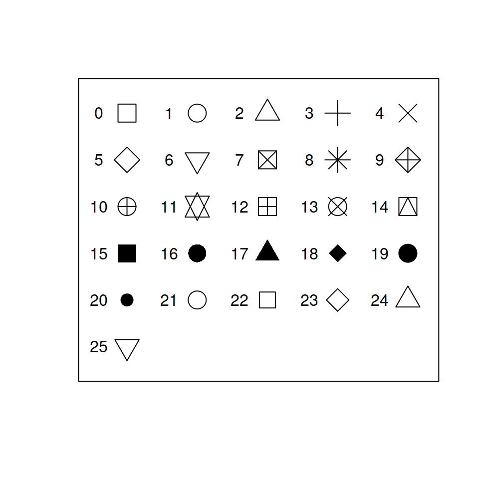
3.  `pch` sets the <a
    href="https://r-charts.com/en/tags/base-r/pch-symbols_files/figure-html/pch-symbols.png"
    data-preview-link="true">type of point</a> used.
4.  `cex` sets the size of the points. The default is 1.
5.  `main` sets the title of the plot. The default is blank.
6.  `xlab` sets the name of the x-axis. The default is the vector name
    you gave the function.
7.  `ylab` sets the name of the y-axis. The default is the vector name
    you gave the function.

Try exploring some of these options by yourself:

``` r
plot(ford$mileage, ford$cost_per_mile,
     las = 1, pch = , cex = ,
     col = "",
     main = "",
     xlab = "",
     ylab = "")
```

Below, I have provided a working example.

<details class="code-fold">
<summary>Code</summary>

``` r
plot(ford$mileage, ford$cost_per_mile, las = 1,
     pch = 23, cex = 1.2,
     col = "tomato", main = "Cost vs Mileage",
     xlab = "Mileage", ylab = "Price per Mile")
```

</details>

<details>

<summary>

Plot
</summary>

<img src="module01_img/01-01-unnamed-chunk-31-1.svg" style="width:90.0%"
data-fig-align="center" data-fig-alt="Mileage vs Cost per Mile" />

</details>

### Adding Lines

We can also add reference lines with the `abline()` function. If you
want a horizontal line at some value `y`, you could use `abline(h = y)`.
If you wanted the line to be vertical, you would use `v =` instead of
`h =`. To use `abline()`, you much first have the plot axes set up.
Remember, R plots are just layers.

### Colors

We can also make the colors a bit more complex. Remember how we used
logic with the `diamond` data to subset it? We can do the same thing
with coloring in graphs. Let’s color the points of older vehicles blue
and newer ones red.

``` r
# If the Year is less than the mean year, color it "dodgerblue"
plot(ford$mileage, ford$cost_per_mile, las = 1,
     pch = 19, cex = 1.2, main = "Cost vs Mileage",
     col = ifelse(ford$year < mean(ford$year), "dodgerblue", "tomato"),
     xlab = "Mileage", ylab = "Price per Mile")
```

<details>

<summary>

Plot
</summary>

<img src="module01_img/01-01-unnamed-chunk-32-1.svg" style="width:90.0%"
data-fig-align="center" data-fig-alt="Mileage vs Cost per Mile" />

</details>

Before moving on, it can be helpful to add opacity to what you plot.
Sometimes, figures can get busy and crowded, so transparency can help us
see where clusters of points are located. To do this, we need to load in
the `scales` package like we did before. Then, when using the `col`
argument, we will use `alpha("tomato", 0.3)`. The first part of this,
where we have `"tomato"`, can be a vector of colors. We can even use our
`ifelse()` colors in this slot. The second argument is the opacity,
which is a measure of transparency. A value of 1 means completely solid,
and a value of 0 means invisible. You can play with opacity in the chunk
below:

``` r
colorz <- ifelse(ford$year < mean(ford$year), "dodgerblue", "tomato")
plot(ford$mileage, ford$cost_per_mile, las = 1,
     pch = 19, cex = 1.2, main = "Cost vs Mileage",
     col = alpha(colorz, 0.3),
     xlab = "Mileage", ylab = "Price per Mile")
```

### Legends

Of course, whenever you choose to add some differences in shapes,
colors, etc., it’s helpful to add a legend to your plot. To do this, we
can use the `legend()` function. This function accepts a few important
arguments:

- `x`, `y`: You can specify the exact coordinates of your legend, or you
  can specify things like: `"topleft"`, `"topright"`, `"bottomleft"`, or
  `"bottomright"`.
- `horiz`: this accepts a boolean value, and turns the legend from
  vertical to horizontal.
- `bty`: setting this to `"n"` removes the box around the legend. I
  *always* use this option.
- `legend`: this is the actual text to be displayed in the legend. It
  accepts a character vector, so if you colored your plot by men and
  women, you would use `c("Men", "Women")`.
- `col`: this should match the `legend` option, but is the corresponding
  color for each legend element.
- Then, you will need to specify either `pch` or `lty` options to tell R
  if you want to display points or lines next to your legend. The
  vectors of `pch` or `lty`, like `col`, should match the elements in
  `legend`.

Try creating your own legend in the code chunk below:

``` r
plot(ford$mileage, ford$cost_per_mile, las = 1,
     pch = 19, cex = 1.2, main = "Cost vs Mileage",
     col = ifelse(ford$year < mean(ford$year), "dodgerblue", "tomato"),
     xlab = "Mileage", ylab = "Price per Mile")
legend()
```

### Points

When generating figures, you will sometimes need to add data from a
different source to the same set of axes. As an example, let’s simply
plot the data above, but in two steps instead of one.

To do this, we will use `points()`. This function accepts nearly every
argument `plot()` does, except you are unable to impact the axes/labels
of the plot.

``` r
choose_rows <- ford$year < mean(ford$year)
plot(ford$mileage[choose_rows],
     ford$cost_per_mile[choose_rows], las = 1,
     pch = 19, cex = 1.2, main = "Cost vs Mileage",
     col = "tomato",
     xlab = "Mileage", ylab = "Price per Mile")
points(ford$mileage[!choose_rows],
       ford$cost_per_mile[!choose_rows],
       pch = 19, cex = 1.2, col = "dodgerblue")
```

Once you get the hang of using `plot()` and `points()` in tandem, you’ll
find it convenient that `points()` does not impact the axes. However, to
start, this will be annoying. For example, let’s switch the order of the
data in `plot()` and `points()`.

``` r
plot(ford$mileage[!choose_rows],
     ford$cost_per_mile[!choose_rows], las = 1,
     pch = 19, cex = 1.2, main = "Cost vs Mileage",
     col = "dodgerblue",
     xlab = "Mileage", ylab = "Price per Mile")
points(ford$mileage[choose_rows],
       ford$cost_per_mile[choose_rows],
       pch = 19, cex = 1.2, col = "tomato")
```

The plot is different because when `plot()` is setting the axes, it
doesn’t know that you’re planning on using `points()` next. So, it
scales the axes so the data fed into `plot()` “fits” the space. Once
again: layers.

To overcome this, we can use the following trick. We are going to set up
our axes before we plot anything. We can do this using `range()`. Try
playing with some of the code below:

``` r
plot(0, 0, type = "n", las = 1,
     # range can include multiple vectors
     ylim = range(ford$cost_per_mile),
     xlim = range(ford$mileage),
     main = "Cost vs Mileage",
     xlab = "Mileage", ylab = "Price per Mile")
points(ford$mileage[!choose_rows],
       ford$cost_per_mile[!choose_rows],
       pch = 19, cex = 1.2, col = "dodgerblue")
points(ford$mileage[choose_rows],
       ford$cost_per_mile[choose_rows],
       col = "tomato")
```

Of course, this is a *lot* more coding than the initial plot’s code. The
idea of showing you this is that, now, you can always make sure your
data “fits”. This is one of the little things that I use constantly, but
it took me a long time to figure out.

### Lines

Finally, adding lines to a plot is very similar in that one needs to use
`lines()`. To illustrate, we will examine [panel data on cigarette
consumption by
state](https://vincentarelbundock.github.io/Rdatasets/csv/Ecdat/Cigar.csv)
([documentation](https://vincentarelbundock.github.io/Rdatasets/doc/Ecdat/Cigar.html)).

Read in the data, inspect it a bit, and then plot sales by year.

``` r
cig <- read.csv()
cig$year <- cig$year + 1900
plot()
```

This figure might be difficult to understand. Let’s trim it down to just
a few states.[^1] In addition, color the points differently by state.

``` r
choose_rows <- cig$state %in% 1:5
plot(
     # since state is a number,
     #  we can just use this as the color
     col = cig$state[choose_rows])
```

This plot can still be improved. It’d be a lot more natural to see the
data as lines instead of points. To do this, we can use `type = "l"`.
Recreate the plot above, but change the plot type.

Notice two things about this plot. First, there’s only a single color.
In R, you should think of a line as a single point. R cannot color
different parts of line differently, so it will just take the first
color (here, it’s 1, which is black). Second, there are these insane
diagonal lines across the plot. This is because R wants to connect
everything into a single line.

To fix this, we need to use `lines()` like we used `points()` before.
This is an example case of a time where we’ll want to set up the axes
before we plot anything.

<details class="code-fold">
<summary>Code</summary>

``` r
# before, I plotted 0, 0
# now, I am simply keeping the data
#   in plot().
# this way, I don't need to set the axes
#   via ylim() and xlim()
plot(cig$year[choose_rows], cig$sales[choose_rows],
     las = 1, type = "n",
     ylab = "Sales", xlab = "Year")
lines(cig$year[cig$state == 1],
      cig$sales[cig$state == 1],
      col = 1)
# Skipping 2 because it doesn't exist
lines(cig$year[cig$state == 3],
      cig$sales[cig$state == 3],
      col = 3)
lines(cig$year[cig$state == 4],
      cig$sales[cig$state == 4],
      col = 4)
lines(cig$year[cig$state == 5],
      cig$sales[cig$state == 5],
      col = 5)
legend("bottomleft", ncol = 2,
       legend = c("State 1", "State 3", "State 4", "State 5"),
       bty = "n", col = c(1, 3, 4, 5), lty = 1)
```

</details>

<details>

<summary>

Plot
</summary>

<img src="module01_img/01-01-unnamed-chunk-41-1.svg" style="width:90.0%"
data-fig-align="center"
data-fig-alt="A correct time series plot of the first four states, each colored differently." />

</details>

This can also be done via looping. Try finishing the following code:

``` r
plot(cig$year[choose_rows], cig$sales[choose_rows],
     las = 1, type = "n",
     ylab = "Sales", xlab = "Year")

for(i in c(1, 3, 4, 5)){
  
  lines()
}

legend("bottomleft", ncol = 2,
       legend = c("State 1", "State 3", "State 4", "State 5"),
       bty = "n", col = c(1, 3, 4, 5), lty = 1)
```

[^1]: Unfortunately, the states seem to just be numbered instead of
    labeled, so we’ll just pick 1 through 5. In addition, note that
    there does not seem to be a state number 2.